GNU Scientific Library
Reference Manual
Edition 1.0, for GSL Version 1.0
1 November 2001
Mark Galassi
Jim Davies
James Theiler
Brian Gough
Gerard Jungman
Michael Booth
Fabrice Rossi
@raggedbottom
@dircategory Scientific software
* gsl-ref: (gsl-ref). GNU Scientific Library -- Reference
Los Alamos National Laboratory
Department of Computer Science, Georgia Institute of Technology
Astrophysics and Radiation Measurements Group, Los Alamos National Laboratory
Network Theory Limited
Theoretical Fluid Dynamics Group, Los Alamos National Laboratory
Department of Physics and Astronomy, The Johns Hopkins University
University of Paris-Dauphine
Copyright (C) 1996, 1997, 1998, 1999, 2000, 2001 The GSL Team.
Permission is granted to copy, distribute and/or modify this document
under the terms of the GNU Free Documentation License, Version 1.1
or any later version published by the Free Software Foundation;
with no Invariant Sections, no Front-Cover Texts, and no Back-Cover Texts.
A copy of the license is included in the section entitled "GNU
Free Documentation License".
The GNU Scientific Library (GSL) is a collection of routines for
numerical computing. The routines have been written from scratch in C,
and are meant to present a modern Applications Programming Interface
(API) for C programmers, while allowing wrappers to be written for very
high level languages. The source code is distributed under the GNU
General Public License.
The library covers a wide range of topics in numerical computing.
Routines are available for the following areas,
| Complex Numbers | Roots of Polynomials |
| Special Functions | Vectors and Matrices |
| Permutations | Sorting |
| BLAS Support | Linear Algebra |
| Eigensystems | Fast Fourier Transforms |
| Quadrature | Random Numbers |
| Quasi-Random Sequences | Random Distributions |
| Statistics | Histograms |
| N-Tuples | Monte Carlo Integration |
| Simulated Annealing | Differential Equations |
| Interpolation | Numerical Differentiation |
| Chebyshev Approximations | Series Acceleration |
| Discrete Hankel Transforms | Root-Finding |
| Minimization | Least-Squares Fitting |
| Physical Constants | IEEE Floating-Point |
The use of these routines is described in this manual. Each chapter
provides detailed definitions of the functions, followed by example
programs and references to the articles on which the algorithms are
based.
The subroutines in the GNU Scientific Library are "free software";
this means that everyone is free to use them, and to redistribute them
in other free programs. The library is not in the public domain; it is
copyrighted and there are conditions on its distribution. These
conditions are designed to permit everything that a good cooperating
citizen would want to do. What is not allowed is to try to prevent
others from further sharing any version of the software that they might
get from you.
Specifically, we want to make sure that you have the right to give away
copies of any programs related to the GNU Scientific Library, that you
receive their source code or else can get it if you want it, that you
can change these programs or use pieces of them in new free programs,
and that you know you can do these things. The library should not be
redistributed in proprietary programs.
To make sure that everyone has such rights, we have to forbid you to
deprive anyone else of these rights. For example, if you distribute
copies of any related code, you must give the recipients all the rights
that you have. You must make sure that they, too, receive or can get
the source code. And you must tell them their rights.
Also, for our own protection, we must make certain that everyone finds
out that there is no warranty for the GNU Scientific Library. If these
programs are modified by someone else and passed on, we want their
recipients to know that what they have is not what we distributed, so
that any problems introduced by others will not reflect on our
reputation.
The precise conditions for the distribution of software related to the
GNU Scientific Library are found in the GNU General Public License
(see section GNU General Public License). Further information about this
license is available from the GNU Project webpage Frequently Asked
Questions about the GNU GPL,
The source code for the library can be obtained in different ways, by
copying it from a friend, purchasing it on CDROM or downloading it
from the internet. A list of public ftp servers which carry the source
code can be found on the development website,
The preferred platform for the library is a GNU system, which
allows it to take advantage of additional features. The library is
portable and compiles on most Unix platforms. It is also available for
Microsoft Windows. Precompiled versions of the library can be purchased
from commercial redistributors listed on the website.
Announcements of new releases, updates and other relevant events are
made on the gsl-announce mailing list. To subscribe to this
low-volume list, send an email of the following form,
To: gsl-announce-request@sources.redhat.com
Subject: subscribe
You will receive a response asking to you to reply in order to confirm
your subscription.
The following short program demonstrates the use of the library by
computing the value of the Bessel function J_0(x) for x=5,
#include <stdio.h>
#include <gsl/gsl_sf_bessel.h>

int
main (void)
{
  double x = 5.0;

  double y = gsl_sf_bessel_J0 (x);

  printf("J0(%g) = %.18e\n", x, y);

  return 0;
}
The output is shown below, and should be correct to double-precision
accuracy,
J0(5) = -1.775967713143382920e-01
The steps needed to compile programs which use the library are described
in the next chapter.
The software described in this manual has no warranty, it is provided
"as is". It is your responsibility to validate the behavior of the
routines and their accuracy using the source code provided. Consult the
GNU General Public license for further details (see section GNU General Public License).
Additional information, including online copies of this manual, links to
related projects, and mailing list archives are available from the
development website mentioned above. The developers of the library can
be reached via the project's public mailing list,
gsl-discuss@sources.redhat.com
This mailing list can be used to report bugs or to ask questions not
covered by this manual.
This chapter describes how to compile programs that use GSL, and
introduces its conventions.
The library is written in ANSI C and is intended to conform to the ANSI
C standard. It should be portable to any system with a working ANSI C
compiler.
The library does not rely on any non-ANSI extensions in the interface it
exports to the user. Programs you write using GSL can be ANSI
compliant. Extensions which can be used in a way compatible with pure
ANSI C are supported, however, via conditional compilation. This allows
the library to take advantage of compiler extensions on those platforms
which support them.
When an ANSI C feature is known to be broken on a particular system the
library will exclude any related functions at compile-time. This should
make it impossible to link a program that would use these functions and
give incorrect results.
To avoid namespace conflicts all exported function names and variables
have the prefix gsl_, while exported macros have the prefix
GSL_.
The library header files are installed in their own `gsl'
directory. You should write any preprocessor include statements with a
`gsl/' directory prefix thus,
#include <gsl/gsl_math.h>
If the directory is not installed on the standard search path of your
compiler you will also need to provide its location to the preprocessor
as a command line flag. The default location of the `gsl'
directory is `/usr/local/include/gsl'.
The library is installed as a single file, `libgsl.a'. A shared
version of the library is also installed on systems that support shared
libraries. The default location of these files is
`/usr/local/lib'. To link against the library you need to specify
both the main library and a supporting CBLAS library, which
provides standard basic linear algebra subroutines. A suitable
CBLAS implementation is provided in the library
`libgslcblas.a' if your system does not provide one. The following
example shows how to link an application with the library,
gcc app.o -lgsl -lgslcblas -lm
The following command line shows how you would link the same application
with an alternative blas library called `libcblas',
gcc app.o -lgsl -lcblas -lm
For the best performance an optimized platform-specific CBLAS
library should be used for -lcblas. The library must conform to
the CBLAS standard. The ATLAS package provides a portable
high-performance BLAS library with a CBLAS interface. It is
free software and should be installed for any work requiring fast vector
and matrix operations. The following command line will link with the
ATLAS library and its CBLAS interface,
gcc app.o -lgsl -lcblas -latlas -lm
For more information see section BLAS Support.
The program gsl-config provides information on the local version
of the library. For example, the following command shows that the
library has been installed under the directory `/usr/local',
bash$ gsl-config --prefix
/usr/local
Further information is available using the command gsl-config --help.
To run a program linked with the shared version of the library it may be
necessary to define the shell variable LD_LIBRARY_PATH to include
the directory where the library is installed. For example,
LD_LIBRARY_PATH=/usr/local/lib:$LD_LIBRARY_PATH ./app
To compile a statically linked version of the program instead, use the
-static flag in gcc,
gcc -static app.o -lgsl -lgslcblas -lm
For applications using autoconf the standard macro
AC_CHECK_LIB can be used to link with the library automatically
from a configure script. The library itself depends on the
presence of a CBLAS and math library as well, so these must also be
located before linking with the main libgsl file. The following
commands should be placed in the `configure.in' file to perform
these tests,
AC_CHECK_LIB(m,main)
AC_CHECK_LIB(gslcblas,main)
AC_CHECK_LIB(gsl,main)
Assuming the libraries are found the output during the configure stage
looks like this,
checking for main in -lm... yes
checking for main in -lgslcblas... yes
checking for main in -lgsl... yes
If the library is found then the tests will define the macros
HAVE_LIBGSL, HAVE_LIBGSLCBLAS, HAVE_LIBM and add
the options -lgsl -lgslcblas -lm to the variable LIBS.
The tests above will find any version of the library. They are suitable
for general use, where the versions of the functions are not important.
An alternative macro is available in the file `gsl.m4' to test for
a specific version of the library. To use this macro simply add the
following line to your `configure.in' file instead of the tests
above:
AM_PATH_GSL(GSL_VERSION,
           [action-if-found],
           [action-if-not-found])
The argument GSL_VERSION should be the two or three digit
MAJOR.MINOR or MAJOR.MINOR.MICRO version number of the release
you require. A suitable choice for action-if-not-found is,
AC_MSG_ERROR(could not find required version of GSL)
Then you can add the variables GSL_LIBS and GSL_CFLAGS to
your Makefile.am files to obtain the correct compiler flags.
GSL_LIBS is equal to the output of the gsl-config --libs
command and GSL_CFLAGS is equal to gsl-config --cflags
command. For example,
libgsdv_la_LDFLAGS =    \
        $(GTK_LIBDIR) \
        $(GTK_LIBS) -lgsdvgsl $(GSL_LIBS) -lgslcblas
Note that the macro AM_PATH_GSL needs to use the C compiler so it
should appear in the `configure.in' file before the macro
AC_LANG_CPLUSPLUS for programs that use C++.
The inline keyword is not part of ANSI C and the library does not
export any inline function definitions by default. However, the library
provides optional inline versions of performance-critical functions by
conditional compilation. The inline versions of these functions can be
included by defining the macro HAVE_INLINE when compiling an
application.
gcc -c -DHAVE_INLINE app.c
If you use autoconf this macro can be defined automatically.
The following test should be placed in your `configure.in' file,
AC_C_INLINE

if test "$ac_cv_c_inline" != no ; then
  AC_DEFINE(HAVE_INLINE,1)
  AC_SUBST(HAVE_INLINE)
fi
and the macro will then be defined in the compilation flags or by
including the file `config.h' before any library headers. If you
do not define the macro HAVE_INLINE then the slower non-inlined
versions of the functions will be used instead.
Note that the actual usage of the inline keyword is extern
inline, which eliminates unnecessary function definitions in GCC.
If the form extern inline causes problems with other compilers a
stricter autoconf test can be used, see section Autoconf Macros.
The extended numerical type long double is part of the ANSI C
standard and should be available in every modern compiler. However, the
precision of long double is platform dependent, and this should
be considered when using it. The IEEE standard only specifies the
minimum precision of extended precision numbers, while the precision of
double is the same on all platforms.
In some system libraries the stdio.h formatted input/output
functions printf and scanf are not implemented correctly
for long double. Undefined or incorrect results are avoided by
testing these functions during the configure stage of library
compilation and eliminating certain GSL functions which depend on them
if necessary. The corresponding line in the configure output
looks like this,
checking whether printf works with long double... no
Consequently when long double formatted input/output does not
work on a given system it should be impossible to link a program which
uses GSL functions dependent on this.
If it is necessary to work on a system which does not support formatted
long double input/output then the options are to use binary
formats or to convert long double results into double for
reading and writing.
To help in writing portable applications GSL provides some
implementations of functions that are found in other libraries, such as
the BSD math library. You can write your application to use the native
versions of these functions, and substitute the GSL versions via a
preprocessor macro if they are unavailable on another platform. The
substitution can be made automatically if you use autoconf. For
example, to test whether the BSD function hypot is available you
can include the following line in the configure file `configure.in'
for your application,
AC_CHECK_FUNCS(hypot)
and place the following macro definitions in the file
`config.h.in',
/* Substitute gsl_hypot for missing system hypot */

#ifndef HAVE_HYPOT
#define hypot gsl_hypot
#endif
The application source files can then use the include command
#include <config.h> to substitute gsl_hypot for each
occurrence of hypot when hypot is not available.
In most circumstances the best strategy is to use the native versions of
these functions when available, and fall back to GSL versions otherwise,
since this allows your application to take advantage of any
platform-specific optimizations in the system library. This is the
strategy used within GSL itself.
The main implementation of some functions in the library will not be
optimal on all architectures. For example, there are several ways to
compute a Gaussian random variate and their relative speeds are
platform-dependent. In cases like this the library provides alternate
implementations of these functions with the same interface. If you
write your application using calls to the standard implementation you
can select an alternative version later via a preprocessor definition.
It is also possible to introduce your own optimized functions this way
while retaining portability. The following lines demonstrate the use of
a platform-dependent choice of methods for sampling from the Gaussian
distribution,
#ifdef SPARC
#define gsl_ran_gaussian gsl_ran_gaussian_ratio_method
#endif
#ifdef INTEL
#define gsl_ran_gaussian my_gaussian
#endif
These lines would be placed in the configuration header file
`config.h' of the application, which should then be included by all
the source files. Note that the alternative implementations will not
produce bit-for-bit identical results, and in the case of random number
distributions will produce an entirely different stream of random
variates.
Many functions in the library are defined for different numeric types.
This feature is implemented by varying the name of the function with a
type-related modifier -- a primitive form of C++ templates. The
modifier is inserted into the function name after the initial module
prefix. The following table shows the function names defined for all
the numeric types of an imaginary module gsl_foo with function
fn,
gsl_foo_fn               double
gsl_foo_long_double_fn   long double
gsl_foo_float_fn         float
gsl_foo_long_fn          long
gsl_foo_ulong_fn         unsigned long
gsl_foo_int_fn           int
gsl_foo_uint_fn          unsigned int
gsl_foo_short_fn         short
gsl_foo_ushort_fn        unsigned short
gsl_foo_char_fn          char
gsl_foo_uchar_fn         unsigned char
The normal numeric precision double is considered the default and
does not require a suffix. For example, the function
gsl_stats_mean computes the mean of double precision numbers,
while the function gsl_stats_int_mean computes the mean of
integers.
A corresponding scheme is used for library defined types, such as
gsl_vector and gsl_matrix. In this case the modifier is
appended to the type name. For example, if a module defines a new
type-dependent struct or typedef gsl_foo it is modified for other
types in the following way,
gsl_foo                  double
gsl_foo_long_double      long double
gsl_foo_float            float
gsl_foo_long             long
gsl_foo_ulong            unsigned long
gsl_foo_int              int
gsl_foo_uint             unsigned int
gsl_foo_short            short
gsl_foo_ushort           unsigned short
gsl_foo_char             char
gsl_foo_uchar            unsigned char
When a module contains type-dependent definitions the library provides
individual header files for each type. The filenames are modified as
shown in the below. For convenience the default header includes the
definitions for all the types. To include only the double precision
header, or any other specific type, file use its individual filename.
#include <gsl/gsl_foo.h>               All types
#include <gsl/gsl_foo_double.h>        double
#include <gsl/gsl_foo_long_double.h>   long double
#include <gsl/gsl_foo_float.h>         float
#include <gsl/gsl_foo_long.h>          long
#include <gsl/gsl_foo_ulong.h>         unsigned long
#include <gsl/gsl_foo_int.h>           int
#include <gsl/gsl_foo_uint.h>          unsigned int
#include <gsl/gsl_foo_short.h>         short
#include <gsl/gsl_foo_ushort.h>        unsigned short
#include <gsl/gsl_foo_char.h>          char
#include <gsl/gsl_foo_uchar.h>         unsigned char
The library header files automatically define functions to have
extern "C" linkage when included in C++ programs.
The library assumes that arrays, vectors and matrices passed as
modifiable arguments are not aliased and do not overlap with each other.
This removes the need for the library to handle overlapping memory
regions as a special case, and allows additional optimizations to be
used. If overlapping memory regions are passed as modifiable arguments
then the results of such functions will be undefined. If the arguments
will not be modified (for example, if a function prototype declares them
as const arguments) then overlapping or aliased memory regions
can be safely used.
Where possible the routines in the library have been written to avoid
dependencies between modules and files. This should make it possible to
extract individual functions for use in your own applications, without
needing to have the whole library installed. You may need to define
certain macros such as GSL_ERROR and remove some #include
statements in order to compile the files as standalone units. Reuse of
the library code in this way is encouraged, subject to the terms of the
GNU General Public License.
This chapter describes the way that GSL functions report and handle
errors. By examining the status information returned by every function
you can determine whether it succeeded or failed, and if it failed you
can find out what the precise cause of failure was. You can also define
your own error handling functions to modify the default behavior of the
library.
The functions described in this section are declared in the header file
`gsl_errno.h'.
The library follows the thread-safe error reporting conventions of the
POSIX Threads library. Functions return a non-zero error code to
indicate an error and 0 to indicate success.
int status = gsl_function(...)

if (status) { /* an error occurred */
  .....
  /* status value specifies the type of error */
}
The routines report an error whenever they cannot perform the task
requested of them. For example, a root-finding function would return a
non-zero error code if could not converge to the requested accuracy, or
exceeded a limit on the number of iterations. Situations like this are
a normal occurrence when using any mathematical library and you should
check the return status of the functions that you call.
Whenever a routine reports an error the return value specifies the
type of error. The return value is analogous to the value of the
variable errno in the C library. However, the C library's
errno is a global variable, which is not thread-safe (There can
be only one instance of a global variable per program. Different
threads of execution may overwrite errno simultaneously).
Returning the error number directly avoids this problem. The caller can
examine the return code and decide what action to take, including
ignoring the error if it is not considered serious.
The error code numbers are defined in the file `gsl_errno.h'. They
all have the prefix GSL_ and expand to non-zero constant integer
values. Many of the error codes use the same base name as a
corresponding error code in C library. Here are some of the most common
error codes,
- Macro: int GSL_EDOM
-
Domain error; used by mathematical functions when an argument value does
not fall into the domain over which the function is defined (like
EDOM in the C library)
- Macro: int GSL_ERANGE
-
Range error; used by mathematical functions when the result value is not
representable because of overflow or underflow (like ERANGE in the C
library)
- Macro: int GSL_ENOMEM
-
No memory available. The system cannot allocate more virtual memory
because its capacity is full (like ENOMEM in the C library). This error
is reported when a GSL routine encounters problems when trying to
allocate memory with
malloc.
- Macro: int GSL_EINVAL
-
Invalid argument. This is used to indicate various kinds of problems
with passing the wrong argument to a library function (like EINVAL in the C
library).
Here is an example of some code which checks the return value of a
function where an error might be reported,
int status = gsl_fft_complex_radix2_forward (data, n);

if (status) {
  if (status == GSL_EINVAL) {
     fprintf (stderr, "invalid argument, n=%d\n", n);
  } else {
     fprintf (stderr, "failed, gsl_errno=%d\n",
                      status);
  }
  exit (-1);
}
The function gsl_fft_complex_radix2 only accepts integer lengths
which are a power of two. If the variable n is not a power
of two then the call to the library function will return
GSL_EINVAL, indicating that the length argument is invalid. The
else clause catches any other possible errors.
The error codes can be converted into an error message using the
function gsl_strerror.
- Function: const char * gsl_strerror (const int gsl_errno)
-
This function returns a pointer to a string describing the error code
gsl_errno. For example,
printf("error: %s\n", gsl_strerror (status));
would print an error message like error: output range error for a
status value of GSL_ERANGE.
In addition to reporting errors the library also provides an optional
error handler. The error handler is called by library functions when
they report an error, just before they return to the caller. The
purpose of the handler is to provide a function where a breakpoint can
be set that will catch library errors when running under the debugger.
It is not intended for use in production programs, which should handle
any errors using the error return codes described above.
The default behavior of the error handler is to print a short message
and call abort() whenever an error is reported by the library.
If this default is not turned off then any program using the library
will stop with a core-dump whenever a library routine reports an error.
This is intended as a fail-safe default for programs which do not check
the return status of library routines (we don't encourage you to write
programs this way). If you turn off the default error handler it is
your responsibility to check the return values of the GSL routines. You
can customize the error behavior by providing a new error handler. For
example, an alternative error handler could log all errors to a file,
ignore certain error conditions (such as underflows), or start the
debugger and attach it to the current process when an error occurs.
All GSL error handlers have the type gsl_error_handler_t, which is
defined in `gsl_errno.h',
- Data Type: gsl_error_handler_t
-
This is the type of GSL error handler functions. An error handler will
be passed four arguments which specify the reason for the error (a
string), the name of the source file in which it occurred (also a
string), the line number in that file (an integer) and the error number
(an integer). The source file and line number are set at compile time
using the __FILE__ and __LINE__ directives in the
preprocessor. An error handler function returns type void.
Error handler functions should be defined like this,
void handler (const char * reason,
              const char * file,
              int line,
              int gsl_errno)
To request the use of your own error handler you need to call the
function gsl_set_error_handler which is also declared in
`gsl_errno.h',
- Function: gsl_error_handler_t gsl_set_error_handler (gsl_error_handler_t new_handler)
-
This functions sets a new error handler, new_handler, for the GSL
library routines. The previous handler is returned (so that you can
restore it later). Note that the pointer to a user defined error
handler function is stored in a static variable, so there can only be
one error handler per program. This function should be not be used in
multi-threaded programs except to set up a program-wide error handler
from a master thread. The following example shows how to set and
restore a new error handler,
/* save original handler, install new handler */
old_handler = gsl_set_error_handler (&my_handler);

/* code uses new handler */
.....

/* restore original handler */
gsl_set_error_handler (old_handler);
To use the default behavior (abort on error) set the error
handler to NULL,
old_handler = gsl_set_error_handler (NULL);
- Function: gsl_error_handler_t gsl_set_error_handler_off ()
-
This function turns off the error handler by defining an error handler
which does nothing. This will cause the program to continue after any
error, so the return values from any library routines must be checked.
This is the recommended behavior for production programs. The previous
handler is returned (so that you can restore it later).
The error behavior can be changed for specific applications by
recompiling the library with a customized definition of the
GSL_ERROR macro in the file `gsl_errno.h'.
If you are writing numerical functions in a program which also uses GSL
code you may find it convenient to adopt the same error reporting
conventions as in the library.
To report an error you need to call the function gsl_error with a
string describing the error and then return an appropriate error code
from gsl_errno.h, or a special value, such as NaN. For
convenience the file `gsl_errno.h' defines two macros which carry
out these steps:
- Macro: GSL_ERROR (reason, gsl_errno)
-
This macro reports an error using the GSL conventions and returns a
status value of gsl_errno. It expands to the following code fragment,
gsl_error (reason, __FILE__, __LINE__, gsl_errno);
return gsl_errno;
The macro definition in `gsl_errno.h' actually wraps the code
in a do { ... } while (0) block to prevent possible
parsing problems.
Here is an example of how the macro could be used to report that a
routine did not achieve a requested tolerance. To report the error the
routine needs to return the error code GSL_ETOL.
if (residual > tolerance)
  {
    GSL_ERROR("residual exceeds tolerance", GSL_ETOL);
  }
- Macro: GSL_ERROR_VAL (reason, gsl_errno, value)
-
This macro is the same as GSL_ERROR but returns a user-defined
status value of value instead of an error code. It can be used for
mathematical functions that return a floating point value.
Here is an example where a function needs to return a NaN because
of a mathematical singularity,
if (x == 0)
  {
    GSL_ERROR_VAL("argument lies on singularity",
                  GSL_ERANGE, GSL_NAN);
  }
This chapter describes basic mathematical functions. Some of these
functions are present in system libraries, but the alternative versions
given here can be used as a substitute when the system functions are not
available.
The functions and macros described in this chapter are defined in the
header file `gsl_math.h'.
The library ensures that the standard BSD mathematical constants
are defined. For reference here is a list of the constants.
M_E
-
The base of exponentials, e
M_LOG2E
-
The base-2 logarithm of e, \log_2 (e)
M_LOG10E
-
The base-10 logarithm of e, @c{$\log_{10}(e)$}
\log_10 (e)
M_SQRT2
-
The square root of two, \sqrt 2
M_SQRT1_2
-
The square root of one-half, @c{$\sqrt{1/2}$}
\sqrt{1/2}
M_SQRT3
-
The square root of three, \sqrt 3
M_PI
-
The constant pi, \pi
M_PI_2
-
Pi divided by two, \pi/2
M_PI_4
-
Pi divided by four, \pi/4
M_SQRTPI
-
The square root of pi, \sqrt\pi
M_2_SQRTPI
-
Two divided by the square root of pi, 2/\sqrt\pi
M_1_PI
-
The reciprocal of pi, 1/\pi
M_2_PI
-
Twice the reciprocal of pi, 2/\pi
M_LN10
-
The natural logarithm of ten, \ln(10)
M_LN2
-
The natural logarithm of two, \ln(2)
M_LNPI
-
The natural logarithm of pi, \ln(\pi)
M_EULER
-
Euler's constant, \gamma
- Macro: GSL_POSINF
-
This macro contains the IEEE representation of positive infinity,
+\infty. It is computed from the expression
+1.0/0.0.
- Macro: GSL_NEGINF
-
This macro contains the IEEE representation of negative infinity,
-\infty. It is computed from the expression
-1.0/0.0.
- Macro: GSL_NAN
-
This macro contains the IEEE representation of the Not-a-Number symbol,
NaN. It is computed from the ratio 0.0/0.0.
- Function: int gsl_isnan (const double x)
-
This function returns 1 if x is not-a-number.
- Function: int gsl_isinf (const double x)
-
This function returns +1 if x is positive infinity,
-1 if x is negative infinity and 0 otherwise.
- Function: int gsl_finite (const double x)
-
This function returns 1 if x is a real number, and 0 if it is
infinite or not-a-number.
The following routines provide portable implementations of functions
found in the BSD math library. When native versions are not available
the functions described here can be used instead. The substitution can
be made automatically if you use autoconf to compile your
application (see section Portability functions).
- Function: double gsl_log1p (const double x)
-
This function computes the value of \log(1+x) in a way that is
accurate for small x. It provides an alternative to the BSD math
function
log1p(x).
- Function: double gsl_expm1 (const double x)
-
This function computes the value of \exp(x)-1 in a way that is
accurate for small x. It provides an alternative to the BSD math
function
expm1(x).
- Function: double gsl_hypot (const double x, const double y)
-
This function computes the value of
\sqrt{x^2 + y^2} in a way that avoids overflow. It provides an
alternative to the BSD math function
hypot(x,y).
- Function: double gsl_acosh (const double x)
-
This function computes the value of \arccosh(x). It provides an
alternative to the standard math function
acosh(x).
- Function: double gsl_asinh (const double x)
-
This function computes the value of \arcsinh(x). It provides an
alternative to the standard math function
asinh(x).
- Function: double gsl_atanh (const double x)
-
This function computes the value of \arctanh(x). It provides an
alternative to the standard math function
atanh(x).
A common complaint about the standard C library is its lack of a
function for calculating (small) integer powers. GSL provides a simple
functions to fill this gap. For reasons of efficiency, these functions
do not check for overflow or underflow conditions.
- Function: double gsl_pow_int (double x, int n)
-
This routine computes the power x^n for integer n. The
power is computed using the minimum number of multiplications. For
example, x^8 is computed as ((x^2)^2)^2, requiring only 3
multiplications. A version of this function which also computes the
numerical error in the result is available as
gsl_sf_pow_int_e.
- Function: double gsl_pow_2 (const double x)
-
- Function: double gsl_pow_3 (const double x)
-
- Function: double gsl_pow_4 (const double x)
-
- Function: double gsl_pow_5 (const double x)
-
- Function: double gsl_pow_6 (const double x)
-
- Function: double gsl_pow_7 (const double x)
-
- Function: double gsl_pow_8 (const double x)
-
- Function: double gsl_pow_9 (const double x)
-
These functions can be used to compute small integer powers x^2,
x^3, etc. efficiently. The functions will be inlined when
possible so that use of these functions should be as efficient as
explicitly writing the corresponding product expression.
#include <gsl/gsl_math.h>
double y = gsl_pow_4 (3.141)  /* compute 3.141**4 */
- Macro: GSL_SIGN (x)
-
This macro returns the sign of x. It is defined as
((x) >= 0
? 1 : -1)
. Note that with this definition the sign of zero is positive
(regardless of its IEEE sign bit).
- Macro: GSL_IS_ODD (n)
-
This macro evaluates to 1 if n is odd and 0 if n is
even. The argument n must be of integer type.
- Macro: GSL_IS_EVEN (n)
-
This macro is the opposite of
GSL_IS_ODD(n). It evaluates to 1 if
n is even and 0 if n is odd. The argument n must be of
integer type.
- Macro: GSL_MAX (a, b)
-
This macro returns the maximum of a and b. It is defined as
((a) > (b) ? (a):(b)).
- Macro: GSL_MIN (a, b)
-
This macro returns the minimum of a and b. It is defined as
((a) < (b) ? (a):(b)).
- Function: extern inline double GSL_MAX_DBL (double a, double b)
-
This function returns the maximum of the double precision numbers
a and b using an inline function. The use of a function
allows for type checking of the arguments as an extra safety feature. On
platforms where inline functions are not available the macro
GSL_MAX will be automatically substituted.
- Function: extern inline double GSL_MIN_DBL (double a, double b)
-
This function returns the minimum of the double precision numbers
a and b using an inline function. The use of a function
allows for type checking of the arguments as an extra safety feature. On
platforms where inline functions are not available the macro
GSL_MIN will be automatically substituted.
- Function: extern inline int GSL_MAX_INT (int a, int b)
-
- Function: extern inline int GSL_MIN_INT (int a, int b)
-
These functions return the maximum or minimum of the integers a
and b using an inline function. On platforms where inline
functions are not available the macros
GSL_MAX or GSL_MIN
will be automatically substituted.
- Function: extern inline long double GSL_MAX_LDBL (long double a, long double b)
-
- Function: extern inline long double GSL_MIN_LDBL (long double a, long double b)
-
These functions return the maximum or minimum of the long doubles a
and b using an inline function. On platforms where inline
functions are not available the macros
GSL_MAX or GSL_MIN
will be automatically substituted.
The functions described in this chapter provide support for complex
numbers. The algorithms take care to avoid unnecessary intermediate
underflows and overflows, allowing the functions to evaluated over the
as much of the complex plane as possible.
For multiple-valued functions the branch cuts have been chosen to follow
the conventions of Abramowitz and Stegun in the Handbook of
Mathematical Functions. The functions return principal values which are
the same as those in GNU Calc, which in turn are the same as those in
Common Lisp, The Language (Second Edition) (n.b. The second
edition uses different definitions from the first edition) and the
HP-28/48 series of calculators.
The complex types are defined in the header file `gsl_complex.h',
while the corresponding complex functions and arithmetic operations are
defined in `gsl_complex_math.h'.
Complex numbers are represented using the type gsl_complex. The
internal representation of this type may vary across platforms and
should not be accessed directly. The functions and macros described
below allow complex numbers to be manipulated in a portable way.
For reference, the default form of the gsl_complex type is
given by the following struct,
typedef struct
{
  double dat[2];
} gsl_complex;
The real and imaginary part are stored in contiguous elements of a two
element array. This eliminates any padding between the real and
imaginary parts, dat[0] and dat[1], allowing the struct to
be mapped correctly onto packed complex arrays.
- Function: gsl_complex gsl_complex_rect (double x, double y)
-
This function uses the rectangular cartesian components
(x,y) to return the complex number z = x + i y.
- Function: gsl_complex gsl_complex_polar (double r, double theta)
-
This function returns the complex number z = r \exp(i \theta) = r
(\cos(\theta) + i \sin(\theta)) from the polar representation
(r,theta).
- Macro: GSL_REAL (z)
-
- Macro: GSL_IMAG (z)
-
These macros return the real and imaginary parts of the complex number
z.
- Macro: GSL_SET_COMPLEX (zp, x, y)
-
This macro uses the cartesian components (x,y) to set the
real and imaginary parts of the complex number pointed to by zp.
For example,
GSL_SET_COMPLEX(&z, 3, 4)
sets z to be 3 + 4i.
- Macro: GSL_SET_REAL (zp,x)
-
- Macro: GSL_SET_IMAG (zp,y)
-
These macros allow the real and imaginary parts of the complex number
pointed to by zp to be set independently.
- Function: double gsl_complex_arg (gsl_complex z)
-
This function returns the argument of the complex number z,
\arg(z), where @c{$-\pi < \arg(z) \leq \pi$}
-\pi < \arg(z) <= \pi.
- Function: double gsl_complex_abs (gsl_complex z)
-
This function returns the magnitude of the complex number z, |z|.
- Function: double gsl_complex_abs2 (gsl_complex z)
-
This function returns the squared magnitude of the complex number
z, |z|^2.
- Function: double gsl_complex_logabs (gsl_complex z)
-
This function returns the natural logarithm of the magnitude of the
complex number z, \log|z|. It allows an accurate
evaluation of \log|z| when |z| is close to one. The direct
evaluation of
log(gsl_complex_abs(z)) would lead to a loss of
precision in this case.
- Function: gsl_complex gsl_complex_add (gsl_complex a, gsl_complex b)
-
This function returns the sum of the complex numbers a and
b, z=a+b.
- Function: gsl_complex gsl_complex_sub (gsl_complex a, gsl_complex b)
-
This function returns the difference of the complex numbers a and
b, z=a-b.
- Function: gsl_complex gsl_complex_mul (gsl_complex a, gsl_complex b)
-
This function returns the product of the complex numbers a and
b, z=ab.
- Function: gsl_complex gsl_complex_div (gsl_complex a, gsl_complex b)
-
This function returns the quotient of the complex numbers a and
b, z=a/b.
- Function: gsl_complex gsl_complex_add_real (gsl_complex a, double x)
-
This function returns the sum of the complex number a and the
real number x, z=a+x.
- Function: gsl_complex gsl_complex_sub_real (gsl_complex a, double x)
-
This function returns the difference of the complex number a and the
real number x, z=a-x.
- Function: gsl_complex gsl_complex_mul_real (gsl_complex a, double x)
-
This function returns the product of the complex number a and the
real number x, z=ax.
- Function: gsl_complex gsl_complex_div_real (gsl_complex a, double x)
-
This function returns the quotient of the complex number a and the
real number x, z=a/x.
- Function: gsl_complex gsl_complex_add_imag (gsl_complex a, double y)
-
This function returns the sum of the complex number a and the
imaginary number iy, z=a+iy.
- Function: gsl_complex gsl_complex_sub_imag (gsl_complex a, double y)
-
This function returns the difference of the complex number a and the
imaginary number iy, z=a-iy.
- Function: gsl_complex gsl_complex_mul_imag (gsl_complex a, double y)
-
This function returns the product of the complex number a and the
imaginary number iy, z=a*(iy).
- Function: gsl_complex gsl_complex_div_imag (gsl_complex a, double y)
-
This function returns the quotient of the complex number a and the
imaginary number iy, z=a/(iy).
- Function: gsl_complex gsl_complex_conjugate (gsl_complex z)
-
This function returns the complex conjugate of the complex number
z, z^* = x - i y.
- Function: gsl_complex gsl_complex_inverse (gsl_complex z)
-
This function returns the inverse, or reciprocal, of the complex number
z, 1/z = (x - i y)/(x^2 + y^2).
- Function: gsl_complex gsl_complex_negative (gsl_complex z)
-
This function returns the negative of the complex number
z, -z = (-x) + i(-y).
- Function: gsl_complex gsl_complex_sqrt (gsl_complex z)
-
This function returns the square root of the complex number z,
\sqrt z. The branch cut is the negative real axis. The result
always lies in the right half of the complex plane.
- Function: gsl_complex gsl_complex_sqrt_real (double x)
-
This function returns the complex square root of the real number
x, where x may be negative.
- Function: gsl_complex gsl_complex_pow (gsl_complex z, gsl_complex a)
-
The function returns the complex number z raised to the complex
power a, z^a. This is computed as \exp(\log(z)*a)
using complex logarithms and complex exponentials.
- Function: gsl_complex gsl_complex_pow_real (gsl_complex z, double x)
-
This function returns the complex number z raised to the real
power x, z^x.
- Function: gsl_complex gsl_complex_exp (gsl_complex z)
-
This function returns the complex exponential of the complex number
z, \exp(z).
- Function: gsl_complex gsl_complex_log (gsl_complex z)
-
This function returns the complex natural logarithm (base e) of
the complex number z, \log(z). The branch cut is the
negative real axis.
- Function: gsl_complex gsl_complex_log10 (gsl_complex z)
-
This function returns the complex base-10 logarithm of
the complex number z, @c{$\log_{10}(z)$}
\log_10 (z).
- Function: gsl_complex gsl_complex_log_b (gsl_complex z, gsl_complex b)
-
This function returns the complex base-b logarithm of the complex
number z, \log_b(z). This quantity is computed as the ratio
\log(z)/\log(b).
- Function: gsl_complex gsl_complex_sin (gsl_complex z)
-
This function returns the complex sine of the complex number z,
\sin(z) = (\exp(iz) - \exp(-iz))/(2i).
- Function: gsl_complex gsl_complex_cos (gsl_complex z)
-
This function returns the complex cosine of the complex number z,
\cos(z) = (\exp(iz) + \exp(-iz))/2.
- Function: gsl_complex gsl_complex_tan (gsl_complex z)
-
This function returns the complex tangent of the complex number z,
\tan(z) = \sin(z)/\cos(z).
- Function: gsl_complex gsl_complex_sec (gsl_complex z)
-
This function returns the complex secant of the complex number z,
\sec(z) = 1/\cos(z).
- Function: gsl_complex gsl_complex_csc (gsl_complex z)
-
This function returns the complex cosecant of the complex number z,
\csc(z) = 1/\sin(z).
- Function: gsl_complex gsl_complex_cot (gsl_complex z)
-
This function returns the complex cotangent of the complex number z,
\cot(z) = 1/\tan(z).
- Function: gsl_complex gsl_complex_arcsin (gsl_complex z)
-
This function returns the complex arcsine of the complex number z,
\arcsin(z). The branch cuts are on the real axis, less than -1
and greater than 1.
- Function: gsl_complex gsl_complex_arcsin_real (double z)
-
This function returns the complex arcsine of the real number z,
\arcsin(z). For z between -1 and 1, the
function returns a real value in the range (-\pi,\pi]. For
z less than -1 the result has a real part of -\pi/2
and a positive imaginary part. For z greater than 1 the
result has a real part of \pi/2 and a negative imaginary part.
- Function: gsl_complex gsl_complex_arccos (gsl_complex z)
-
This function returns the complex arccosine of the complex number z,
\arccos(z). The branch cuts are on the real axis, less than -1
and greater than 1.
- Function: gsl_complex gsl_complex_arccos_real (double z)
-
This function returns the complex arccosine of the real number z,
\arccos(z). For z between -1 and 1, the
function returns a real value in the range [0,\pi]. For z
less than -1 the result has a real part of \pi/2 and a
negative imaginary part. For z greater than 1 the result
is purely imaginary and positive.
- Function: gsl_complex gsl_complex_arctan (gsl_complex z)
-
This function returns the complex arctangent of the complex number
z, \arctan(z). The branch cuts are on the imaginary axis,
below -i and above i.
- Function: gsl_complex gsl_complex_arcsec (gsl_complex z)
-
This function returns the complex arcsecant of the complex number z,
\arcsec(z) = \arccos(1/z).
- Function: gsl_complex gsl_complex_arcsec_real (double z)
-
This function returns the complex arcsecant of the real number z,
\arcsec(z) = \arccos(1/z).
- Function: gsl_complex gsl_complex_arccsc (gsl_complex z)
-
This function returns the complex arccosecant of the complex number z,
\arccsc(z) = \arcsin(1/z).
- Function: gsl_complex gsl_complex_arccsc_real (double z)
-
This function returns the complex arccosecant of the real number z,
\arccsc(z) = \arcsin(1/z).
- Function: gsl_complex gsl_complex_arccot (gsl_complex z)
-
This function returns the complex arccotangent of the complex number z,
\arccot(z) = \arctan(1/z).
- Function: gsl_complex gsl_complex_sinh (gsl_complex z)
-
This function returns the complex hyperbolic sine of the complex number
z, \sinh(z) = (\exp(z) - \exp(-z))/2.
- Function: gsl_complex gsl_complex_cosh (gsl_complex z)
-
This function returns the complex hyperbolic cosine of the complex number
z, \cosh(z) = (\exp(z) + \exp(-z))/2.
- Function: gsl_complex gsl_complex_tanh (gsl_complex z)
-
This function returns the complex hyperbolic tangent of the complex number
z, \tanh(z) = \sinh(z)/\cosh(z).
- Function: gsl_complex gsl_complex_sech (gsl_complex z)
-
This function returns the complex hyperbolic secant of the complex
number z, \sech(z) = 1/\cosh(z).
- Function: gsl_complex gsl_complex_csch (gsl_complex z)
-
This function returns the complex hyperbolic cosecant of the complex
number z, \csch(z) = 1/\sinh(z).
- Function: gsl_complex gsl_complex_coth (gsl_complex z)
-
This function returns the complex hyperbolic cotangent of the complex
number z, \coth(z) = 1/\tanh(z).
- Function: gsl_complex gsl_complex_arcsinh (gsl_complex z)
-
This function returns the complex hyperbolic arcsine of the
complex number z, \arcsinh(z). The branch cuts are on the
imaginary axis, below -i and above i.
- Function: gsl_complex gsl_complex_arccosh (gsl_complex z)
-
This function returns the complex hyperbolic arccosine of the complex
number z, \arccosh(z). The branch cut is on the real axis,
less than 1.
- Function: gsl_complex gsl_complex_arccosh_real (double z)
-
This function returns the complex hyperbolic arccosine of
the real number z, \arccosh(z).
- Function: gsl_complex gsl_complex_arctanh (gsl_complex z)
-
This function returns the complex hyperbolic arctangent of the complex
number z, \arctanh(z). The branch cuts are on the real
axis, less than -1 and greater than 1.
- Function: gsl_complex gsl_complex_arctanh_real (double z)
-
This function returns the complex hyperbolic arctangent of the real
number z, \arctanh(z).
- Function: gsl_complex gsl_complex_arcsech (gsl_complex z)
-
This function returns the complex hyperbolic arcsecant of the complex
number z, \arcsech(z) = \arccosh(1/z).
- Function: gsl_complex gsl_complex_arccsch (gsl_complex z)
-
This function returns the complex hyperbolic arccosecant of the complex
number z, \arccsch(z) = \arcsin(1/z).
- Function: gsl_complex gsl_complex_arccoth (gsl_complex z)
-
This function returns the complex hyperbolic arccotangent of the complex
number z, \arccoth(z) = \arctanh(1/z).
The implementations of the elementary and trigonometric functions are
based on the following papers,
-
T. E. Hull, Thomas F. Fairgrieve, Ping Tak Peter Tang,
"Implementing Complex Elementary Functions Using Exception
Handling", ACM Transactions on Mathematical Software, Volume 20
(1994), pp 215-244, Corrigenda, p553
-
T. E. Hull, Thomas F. Fairgrieve, Ping Tak Peter Tang,
"Implementing the complex arcsin and arccosine functions using exception
handling", ACM Transactions on Mathematical Software, Volume 23
(1997) pp 299-335
The general formulas and details of branch cuts can be found in the
following books,
-
Abramowitz and Stegun, Handbook of Mathematical Functions,
"Circular Functions in Terms of Real and Imaginary Parts", Formulas
4.3.55--58,
"Inverse Circular Functions in Terms of Real and Imaginary Parts",
Formulas 4.4.37--39,
"Hyperbolic Functions in Terms of Real and Imaginary Parts",
Formulas 4.5.49--52,
"Inverse Hyperbolic Functions -- relation to Inverse Circular Functions",
Formulas 4.6.14--19.
-
Dave Gillespie, Calc Manual, Free Software Foundation, ISBN
1-882114-18-3
This chapter describes functions for evaluating and solving polynomials.
There are routines for finding real and complex roots of quadratic and
cubic equations using analytic methods. An iterative polynomial solver
is also available for finding the roots of general polynomials with real
coefficients (of any order). The functions are declared in the header
file gsl_poly.h.
- Function: double gsl_poly_eval (const double c[], const int len, const double x)
-
This function evaluates the polynomial
c[0] + c[1] x + c[2] x^2 + \dots + c[len-1] x^{len-1} using
Horner's method for stability. The function is inlined when possible.
- Function: int gsl_poly_solve_quadratic (double a, double b, double c, double *x0, double *x1)
-
This function finds the real roots of the quadratic equation,
The number of real roots (either zero or two) is returned, and their
locations are stored in x0 and x1. If no real roots are
found then x0 and x1 are not modified. When two real roots
are found they are stored in x0 and x1 in ascending
order. The case of coincident roots is not considered special. For
example (x-1)^2=0 will have two roots, which happen to have
exactly equal values.
The number of roots found depends on the sign of the discriminant
b^2 - 4 a c. This will be subject to rounding and cancellation
errors when computed in double precision, and will also be subject to
errors if the coefficients of the polynomial are inexact. These errors
may cause a discrete change in the number of roots. However, for
polynomials with small integer coefficients the discriminant can always
be computed exactly.
- Function: int gsl_poly_complex_solve_quadratic (double a, double b, double c, gsl_complex *z0, gsl_complex *z1)
-
This function finds the complex roots of the quadratic equation,
The number of complex roots is returned (always two) and the locations
of the roots are stored in z0 and z1. The roots are returned
in ascending order, sorted first by their real components and then by
their imaginary components.
- Function: int gsl_poly_solve_cubic (double a, double b, double c, double *x0, double *x1, double *x2)
-
This function finds the real roots of the cubic equation,
with a leading coefficient of unity. The number of real roots (either
one or three) is returned, and their locations are stored in x0,
x1 and x2. If one real root is found then only x0 is
modified. When three real roots are found they are stored in x0,
x1 and x2 in ascending order. The case of coincident roots
is not considered special. For example, the equation (x-1)^3=0
will have three roots with exactly equal values.
- Function: int gsl_poly_complex_solve_cubic (double a, double b, double c, gsl_complex *z0, gsl_complex *z1, gsl_complex *z2)
-
This function finds the complex roots of the cubic equation,
The number of complex roots is returned (always three) and the locations
of the roots are stored in z0, z1 and z2. The roots
are returned in ascending order, sorted first by their real components
and then by their imaginary components.
The roots of polynomial equations cannot be found analytically beyond
the special cases of the quadratic, cubic and quartic equation. The
algorithm described in this section uses an iterative method to find the
approximate locations of roots of higher order polynomials.
- Function: gsl_poly_complex_workspace * gsl_poly_complex_workspace_alloc (size_t n)
-
This function allocates space for a
gsl_poly_complex_workspace
struct and a workspace suitable for solving a polynomial with n
coefficients using the routine gsl_poly_complex_solve.
The function returns a pointer to the newly allocated
gsl_poly_complex_workspace if no errors were detected, and a null
pointer in the case of error.
- Function: void gsl_poly_complex_workspace_free (gsl_poly_complex_workspace * w)
-
This function frees all the memory associated with the workspace
w.
- Function: int gsl_poly_complex_solve (const double * a, size_t n, gsl_poly_complex_workspace * w, gsl_complex_packed_ptr z)
-
This function computes the roots of the general polynomial
P(x) = a_0 + a_1 x + a_2 x^2 + ... + a_{n-1} x^{n-1} using
balanced-QR reduction of the companion matrix. The parameter n
specifies the length of the coefficient array. The coefficient of the
highest order term must be non-zero. The function requires a workspace
w of the appropriate size. The n-1 roots are returned in
the packed complex array z of length 2(n-1), alternating
real and imaginary parts.
The function returns GSL_SUCCESS if all the roots are found and
GSL_EFAILED if the QR reduction does not converge.
To demonstrate the use of the general polynomial solver we will take the
polynomial P(x) = x^5 - 1 which has the following roots,
The following program will find these roots.
#include <stdio.h>
#include <gsl/gsl_poly.h>

int
main (void)
{
  int i;
  /* coefficient of P(x) =  -1 + x^5  */
  double a[6] = { -1, 0, 0, 0, 0, 1 };
  double z[10];

  gsl_poly_complex_workspace * w
      = gsl_poly_complex_workspace_alloc (6);

  gsl_poly_complex_solve (a, 6, w, z);

  gsl_poly_complex_workspace_free (w);

  for (i = 0; i < 5; i++)
    {
      printf("z%d = %+.18f %+.18f\n",
             i, z[2*i], z[2*i+1]);
    }

  return 0;
}
The output of the program is,
bash$ ./a.out
z0 = -0.809016994374947451 +0.587785252292473137
z1 = -0.809016994374947451 -0.587785252292473137
z2 = +0.309016994374947451 +0.951056516295153642
z3 = +0.309016994374947451 -0.951056516295153642
z4 = +1.000000000000000000 +0.000000000000000000
which agrees with the analytic result, z_n = \exp(2 \pi n i/5).
The balanced-QR method and its error analysis is described in the
following papers.
-
R.S. Martin, G. Peters and J.H. Wilkinson, "The QR Algorithm for Real
Hessenberg Matrices", Numerische Mathematik, 14 (1970), 219--231.
-
B.N. Parlett and C. Reinsch, "Balancing a Matrix for Calculation of
Eigenvalues and Eigenvectors", Numerische Mathematik, 13 (1969),
293--304.
-
A. Edelman and H. Murakami, "Polynomial roots from companion matrix
eigenvalues", Mathematics of Computation, Vol. 64 No. 210
(1995), 763--776.
This chapter describes the GSL special function library. The library
includes routines for calculating the values of Airy functions, Bessel
functions, Clausen functions, Coulomb wave functions, Coupling
coefficients, the Dawson function, Debye functions, Dilogarithms,
Elliptic integrals, Jacobi elliptic functions, Error functions,
Exponential integrals, Fermi-Dirac functions, Gamma functions,
Gegenbauer functions, Hypergeometric functions, Laguerre functions,
Legendre functions and Spherical Harmonics, the Psi (Digamma) Function,
Synchrotron functions, Transport functions, Trigonometric functions and
Zeta functions. Each routine also computes an estimate of the numerical
error in the calculated value of the function.
The functions are declared in individual header files, such as
`gsl_sf_airy.h', `gsl_sf_bessel.h', etc. The complete set of
header files can be included using the file `gsl_sf.h'.
The special functions are available in two calling conventions, a
natural form which returns the numerical value of the function and
an error-handling form which returns an error code. The two types
of function provide alternative ways of accessing the same underlying
code.
The natural form returns only the value of the function and can be
used directly in mathematical expressions.. For example, the following
function call will compute the value of the Bessel function
J_0(x),
double y = gsl_sf_bessel_J0 (x);
There is no way to access an error code or to estimate the error using
this method. To allow access to this information the alternative
error-handling form stores the value and error in a modifiable argument,
gsl_sf_result result;
int status = gsl_sf_bessel_J0_e (x, &result);
The error-handling functions have the suffix _e. The returned
status value indicates error conditions such as overflow, underflow or
loss of precision. If there are no errors the error-handling functions
return GSL_SUCCESS.
The error handling form of the special functions always calculate an
error estimate along with the value of the result. Therefore,
structures are provided for amalgamating a value and error estimate.
These structures are declared in the header file `gsl_sf_result.h'.
The gsl_sf_result struct contains value and error fields.
typedef struct
{
  double val;
  double err;
} gsl_sf_result;
The field val contains the value and the field err contains
an estimate of the absolute error in the value.
In some cases, an overflow or underflow can be detected and handled by a
function. In this case, it may be possible to return a scaling exponent
as well as an error/value pair in order to save the result from
exceeding the dynamic range of the built-in types. The
gsl_sf_result_e10 struct contains value and error fields as well
as an exponent field such that the actual result is obtained as
result * 10^(e10).
typedef struct
{
  double val;
  double err;
  int    e10;
} gsl_sf_result_e10;
The goal of the library is to achieve double precision accuracy wherever
possible. However the cost of evaluating some special functions to
double precision can be significant, particularly where very high order
terms are required. In these cases a mode argument allows the
accuracy of the function to be reduced in order to improve performance.
The following precision levels are available for the mode argument,
GSL_PREC_DOUBLE
-
Double-precision, a relative accuracy of approximately @c{$2 \times 10^{-16}$}
2 * 10^-16.
GSL_PREC_SINGLE
-
Single-precision, a relative accuracy of approximately @c{$1 \times 10^{-7}$}
10^-7.
GSL_PREC_APPROX
-
Approximate values, a relative accuracy of approximately @c{$5 \times 10^{-4}$}
5 * 10^-4.
The approximate mode provides the fastest evaluation at the lowest
accuracy.
The Airy functions Ai(x) and Bi(x) are defined by the
integral representations,
For further information see Abramowitz & Stegun, Section 10.4. The Airy
functions are defined in the header file `gsl_sf_airy.h'.
- Function: double gsl_sf_airy_Ai (double x, gsl_mode_t mode)
-
- Function: int gsl_sf_airy_Ai_e (double x, gsl_mode_t mode, gsl_sf_result * result)
-
These routines compute the Airy function Ai(x) with an accuracy
specified by mode.
- Function: double gsl_sf_airy_Bi (double x, gsl_mode_t mode)
-
- Function: int gsl_sf_airy_Bi_e (double x, gsl_mode_t mode, gsl_sf_result * result)
-
These routines compute the Airy function Bi(x) with an accuracy
specified by mode.
- Function: double gsl_sf_airy_Ai_scaled (double x, gsl_mode_t mode)
-
- Function: int gsl_sf_airy_Ai_scaled_e (double x, gsl_mode_t mode, gsl_sf_result * result)
-
These routines compute a scaled version of the Airy function
S_A(x) Ai(x). For x>0 the scaling factor S_A(x) is @c{$\exp(+(2/3) x^{3/2})$}
\exp(+(2/3) x^(3/2)),
and is 1
for x<0.
- Function: double gsl_sf_airy_Bi_scaled (double x, gsl_mode_t mode)
-
- Function: int gsl_sf_airy_Bi_scaled_e (double x, gsl_mode_t mode, gsl_sf_result * result)
-
These routines compute a scaled version of the Airy function
S_B(x) Bi(x). For x>0 the scaling factor S_B(x) is @c{$\exp(-(2/3) x^{3/2})$}
exp(-(2/3) x^(3/2)), and is 1 for x<0.
- Function: double gsl_sf_airy_Ai_deriv (double x, gsl_mode_t mode)
-
- Function: int gsl_sf_airy_Ai_deriv_e (double x, gsl_mode_t mode, gsl_sf_result * result)
-
These routines compute the Airy function derivative Ai'(x) with
an accuracy specified by mode.
- Function: double gsl_sf_airy_Bi_deriv (double x, gsl_mode_t mode)
-
- Function: int gsl_sf_airy_Bi_deriv_e (double x, gsl_mode_t mode, gsl_sf_result * result)
-
These routines compute the Airy function derivative Bi'(x) with
an accuracy specified by mode.
- Function: double gsl_sf_airy_Ai_deriv_scaled (double x, gsl_mode_t mode)
-
- Function: int gsl_sf_airy_Ai_deriv_scaled_e (double x, gsl_mode_t mode, gsl_sf_result * result)
-
These routines compute the derivative of the scaled Airy
function S_A(x) Ai(x).
- Function: double gsl_sf_airy_Bi_deriv_scaled (double x, gsl_mode_t mode)
-
- Function: int gsl_sf_airy_Bi_deriv_scaled_e (double x, gsl_mode_t mode, gsl_sf_result * result)
-
These routines compute the derivative of the scaled Airy function
S_B(x) Bi(x).
- Function: double gsl_sf_airy_zero_Ai (unsigned int s)
-
- Function: int gsl_sf_airy_zero_Ai_e (unsigned int s, gsl_sf_result * result)
-
These routines compute the location of the s-th zero of the Airy
function Ai(x).
- Function: double gsl_sf_airy_zero_Bi (unsigned int s)
-
- Function: int gsl_sf_airy_zero_Bi_e (unsigned int s, gsl_sf_result * result)
-
These routines compute the location of the s-th zero of the Airy
function Bi(x).
- Function: double gsl_sf_airy_zero_Ai_deriv (unsigned int s)
-
- Function: int gsl_sf_airy_zero_Ai_deriv_e (unsigned int s, gsl_sf_result * result)
-
These routines compute the location of the s-th zero of the Airy
function derivative Ai'(x).
- Function: double gsl_sf_airy_zero_Bi_deriv (unsigned int s)
-
- Function: int gsl_sf_airy_zero_Bi_deriv_e (unsigned int s, gsl_sf_result * result)
-
These routines compute the location of the s-th zero of the Airy
function derivative Bi'(x).
The routines described in this section compute the Cylindrical Bessel
functions J_n(x), Y_n(x), Modified cylindrical Bessel
functions I_n(x), K_n(x), Spherical Bessel functions
j_l(x), y_l(x), and Modified Spherical Bessel functions
i_l(x), k_l(x). For more information see Abramowitz & Stegun,
Chapters 9 and 10. The Bessel functions are defined in the header file
`gsl_sf_bessel.h'.
- Function: double gsl_sf_bessel_J0 (double x)
-
- Function: int gsl_sf_bessel_J0_e (double x, gsl_sf_result * result)
-
These routines compute the regular cylindrical Bessel function of zeroth
order, J_0(x).
- Function: double gsl_sf_bessel_J1 (double x)
-
- Function: int gsl_sf_bessel_J1_e (double x, gsl_sf_result * result)
-
These routines compute the regular cylindrical Bessel function of first
order, J_1(x).
- Function: double gsl_sf_bessel_Jn (int n, double x)
-
- Function: int gsl_sf_bessel_Jn_e (int n, double x, gsl_sf_result * result)
-
These routines compute the regular cylindrical Bessel function of
order n, J_n(x).
- Function: int gsl_sf_bessel_Jn_array (int nmin, int nmax, double x, double result_array[])
-
This routine computes the values of the regular cylindrical Bessel
functions J_n(x) for n from nmin to nmax
inclusive, storing the results in the array result_array. The
values are computed using recurrence relations, for efficiency, and
therefore may differ slightly from the exact values.
- Function: double gsl_sf_bessel_Y0 (double x)
-
- Function: int gsl_sf_bessel_Y0_e (double x, gsl_sf_result * result)
-
These routines compute the irregular cylindrical Bessel function of zeroth
order, Y_0(x), for x>0.
- Function: double gsl_sf_bessel_Y1 (double x)
-
- Function: int gsl_sf_bessel_Y1_e (double x, gsl_sf_result * result)
-
These routines compute the irregular cylindrical Bessel function of first
order, Y_1(x), for x>0.
- Function: double gsl_sf_bessel_Yn (int n,double x)
-
- Function: int gsl_sf_bessel_Yn_e (int n,double x, gsl_sf_result * result)
-
These routines compute the irregular cylindrical Bessel function of
order n, Y_n(x), for x>0.
- Function: int gsl_sf_bessel_Yn_array (int nmin, int nmax, double x, double result_array[])
-
This routine computes the values of the irregular cylindrical Bessel
functions Y_n(x) for n from nmin to nmax
inclusive, storing the results in the array result_array. The
domain of the function is x>0. The values are computed using
recurrence relations, for efficiency, and therefore may differ slightly
from the exact values.
- Function: double gsl_sf_bessel_I0 (double x)
-
- Function: int gsl_sf_bessel_I0_e (double x, gsl_sf_result * result)
-
These routines compute the regular modified cylindrical Bessel function
of zeroth order, I_0(x).
- Function: double gsl_sf_bessel_I1 (double x)
-
- Function: int gsl_sf_bessel_I1_e (double x, gsl_sf_result * result)
-
These routines compute the regular modified cylindrical Bessel function
of first order, I_1(x).
- Function: double gsl_sf_bessel_In (int n, double x)
-
- Function: int gsl_sf_bessel_In_e (int n, double x, gsl_sf_result * result)
-
These routines compute the regular modified cylindrical Bessel function
of order n, I_n(x).
- Function: int gsl_sf_bessel_In_array (int nmin, int nmax, double x, double result_array[])
-
This routine computes the values of the regular modified cylindrical
Bessel functions I_n(x) for n from nmin to
nmax inclusive, storing the results in the array
result_array. The start of the range nmin must be positive
or zero. The values are computed using recurrence relations, for
efficiency, and therefore may differ slightly from the exact values.
- Function: double gsl_sf_bessel_I0_scaled (double x)
-
- Function: int gsl_sf_bessel_I0_scaled_e (double x, gsl_sf_result * result)
-
These routines compute the scaled regular modified cylindrical Bessel
function of zeroth order \exp(-|x|) I_0(x).
- Function: double gsl_sf_bessel_I1_scaled (double x)
-
- Function: int gsl_sf_bessel_I1_scaled_e (double x, gsl_sf_result * result)
-
These routines compute the scaled regular modified cylindrical Bessel
function of first order \exp(-|x|) I_1(x).
- Function: double gsl_sf_bessel_In_scaled (int n, double x)
-
- Function: int gsl_sf_bessel_In_scaled_e (int n, double x, gsl_sf_result * result)
-
These routines compute the scaled regular modified cylindrical Bessel
function of order n, \exp(-|x|) I_n(x)
- Function: int gsl_sf_bessel_In_scaled_array (int nmin, int nmax, double x, double result_array[])
-
This routine computes the values of the scaled regular cylindrical
Bessel functions \exp(-|x|) I_n(x) for n from
nmin to nmax inclusive, storing the results in the array
result_array. The start of the range nmin must be positive
or zero. The values are computed using recurrence relations, for
efficiency, and therefore may differ slightly from the exact values.
- Function: double gsl_sf_bessel_K0 (double x)
-
- Function: int gsl_sf_bessel_K0_e (double x, gsl_sf_result * result)
-
These routines compute the irregular modified cylindrical Bessel
function of zeroth order, K_0(x), for x > 0.
- Function: double gsl_sf_bessel_K1 (double x)
-
- Function: int gsl_sf_bessel_K1_e (double x, gsl_sf_result * result)
-
These routines compute the irregular modified cylindrical Bessel
function of first order, K_1(x), for x > 0.
- Function: double gsl_sf_bessel_Kn (int n, double x)
-
- Function: int gsl_sf_bessel_Kn_e (int n, double x, gsl_sf_result * result)
-
These routines compute the irregular modified cylindrical Bessel
function of order n, K_n(x), for x > 0.
- Function: int gsl_sf_bessel_Kn_array (int nmin, int nmax, double x, double result_array[])
-
This routine computes the values of the irregular modified cylindrical
Bessel functions K_n(x) for n from nmin to
nmax inclusive, storing the results in the array
result_array. The start of the range nmin must be positive
or zero. The domain of the function is x>0. The values are
computed using recurrence relations, for efficiency, and therefore
may differ slightly from the exact values.
- Function: double gsl_sf_bessel_K0_scaled (double x)
-
- Function: int gsl_sf_bessel_K0_scaled_e (double x, gsl_sf_result * result)
-
These routines compute the scaled irregular modified cylindrical Bessel
function of zeroth order \exp(x) K_0(x) for x>0.
- Function: double gsl_sf_bessel_K1_scaled (double x)
-
- Function: int gsl_sf_bessel_K1_scaled_e (double x, gsl_sf_result * result)
-
These routines compute the scaled irregular modified cylindrical Bessel
function of first order \exp(x) K_1(x) for x>0.
- Function: double gsl_sf_bessel_Kn_scaled (int n, double x)
-
- Function: int gsl_sf_bessel_Kn_scaled_e (int n, double x, gsl_sf_result * result)
-
These routines compute the scaled irregular modified cylindrical Bessel
function of order n, \exp(x) K_n(x), for x>0.
- Function: int gsl_sf_bessel_Kn_scaled_array (int nmin, int nmax, double x, double result_array[])
-
This routine computes the values of the scaled irregular cylindrical
Bessel functions \exp(x) K_n(x) for n from nmin to
nmax inclusive, storing the results in the array
result_array. The start of the range nmin must be positive
or zero. The domain of the function is x>0. The values are
computed using recurrence relations, for efficiency, and therefore
may differ slightly from the exact values.
- Function: double gsl_sf_bessel_j0 (double x)
-
- Function: int gsl_sf_bessel_j0_e (double x, gsl_sf_result * result)
-
These routines compute the regular spherical Bessel function of zeroth
order, j_0(x) = \sin(x)/x.
- Function: double gsl_sf_bessel_j1 (double x)
-
- Function: int gsl_sf_bessel_j1_e (double x, gsl_sf_result * result)
-
These routines compute the regular spherical Bessel function of first
order, j_1(x) = (\sin(x)/x - \cos(x))/x.
- Function: double gsl_sf_bessel_j2 (double x)
-
- Function: int gsl_sf_bessel_j2_e (double x, gsl_sf_result * result)
-
These routines compute the regular spherical Bessel function of second
order, j_2(x) = ((3/x^2 - 1)\sin(x) - 3\cos(x)/x)/x.
- Function: double gsl_sf_bessel_jl (int l, double x)
-
- Function: int gsl_sf_bessel_jl_e (int l, double x, gsl_sf_result * result)
-
These routines compute the regular spherical Bessel function of
order l, j_l(x), for @c{$l \geq 0$}
l >= 0 and @c{$x \geq 0$}
x >= 0.
- Function: int gsl_sf_bessel_jl_array (int lmax, double x, double result_array[])
-
This routine computes the values of the regular spherical Bessel
functions j_l(x) for l from 0 to lmax
inclusive for @c{$lmax \geq 0$}
lmax >= 0 and @c{$x \geq 0$}
x >= 0, storing the results in the array result_array.
The values are computed using recurrence relations, for
efficiency, and therefore may differ slightly from the exact values.
- Function: int gsl_sf_bessel_jl_steed_array (int lmax, double x, double * jl_x_array)
-
This routine uses Steed's method to compute the values of the regular
spherical Bessel functions j_l(x) for l from 0 to
lmax inclusive for @c{$lmax \geq 0$}
lmax >= 0 and @c{$x \geq 0$}
x >= 0, storing the results in the array
result_array.
The Steed/Barnett algorithm is described in Comp. Phys. Comm. 21,
297 (1981). Steed's method is more stable than the
recurrence used in the other functions but is also slower.
- Function: double gsl_sf_bessel_y0 (double x)
-
- Function: int gsl_sf_bessel_y0_e (double x, gsl_sf_result * result)
-
These routines compute the irregular spherical Bessel function of zeroth
order, y_0(x) = -\cos(x)/x.
- Function: double gsl_sf_bessel_y1 (double x)
-
- Function: int gsl_sf_bessel_y1_e (double x, gsl_sf_result * result)
-
These routines compute the irregular spherical Bessel function of first
order, y_1(x) = -(\cos(x)/x + \sin(x))/x.
- Function: double gsl_sf_bessel_y2 (double x)
-
- Function: int gsl_sf_bessel_y2_e (double x, gsl_sf_result * result)
-
These routines compute the irregular spherical Bessel function of second
order, y_2(x) = (-3/x^2 + 1/x)\cos(x) - (3/x^2)\sin(x).
- Function: double gsl_sf_bessel_yl (int l, double x)
-
- Function: int gsl_sf_bessel_yl_e (int l, double x, gsl_sf_result * result)
-
These routines compute the irregular spherical Bessel function of
order l, y_l(x), for @c{$l \geq 0$}
l >= 0.
- Function: int gsl_sf_bessel_yl_array (int lmax, double x, double result_array[])
-
This routine computes the values of the irregular spherical Bessel
functions y_l(x) for l from 0 to lmax
inclusive for @c{$lmax \geq 0$}
lmax >= 0, storing the results in the array result_array.
The values are computed using recurrence relations, for
efficiency, and therefore may differ slightly from the exact values.
The regular modified spherical Bessel functions i_l(x)
are related to the modified Bessel functions of fractional order,
i_l(x) = \sqrt{\pi/(2x)} I_{l+1/2}(x)
- Function: double gsl_sf_bessel_i0_scaled (double x)
-
- Function: int gsl_sf_bessel_i0_scaled_e (double x, gsl_sf_result * result)
-
These routines compute the scaled regular modified spherical Bessel
function of zeroth order, \exp(-|x|) i_0(x).
- Function: double gsl_sf_bessel_i1_scaled (double x)
-
- Function: int gsl_sf_bessel_i1_scaled_e (double x, gsl_sf_result * result)
-
These routines compute the scaled regular modified spherical Bessel
function of first order, \exp(-|x|) i_1(x).
- Function: double gsl_sf_bessel_i2_scaled (double x)
-
- Function: int gsl_sf_bessel_i2_scaled_e (double x, gsl_sf_result * result)
-
These routines compute the scaled regular modified spherical Bessel
function of second order, \exp(-|x|) i_2(x)
- Function: double gsl_sf_bessel_il_scaled (int l, double x)
-
- Function: int gsl_sf_bessel_il_scaled_e (int l, double x, gsl_sf_result * result)
-
These routines compute the scaled regular modified spherical Bessel
function of order l, \exp(-|x|) i_l(x)
- Function: int gsl_sf_bessel_il_scaled_array (int lmax, double x, double result_array[])
-
This routine computes the values of the scaled regular modified
cylindrical Bessel functions \exp(-|x|) i_l(x) for l from
0 to lmax inclusive for @c{$lmax \geq 0$}
lmax >= 0, storing the results in
the array result_array.
The values are computed using recurrence relations, for
efficiency, and therefore may differ slightly from the exact values.
The irregular modified spherical Bessel functions k_l(x)
are related to the irregular modified Bessel functions of fractional order,
k_l(x) = \sqrt{\pi/(2x)} K_{l+1/2}(x).
- Function: double gsl_sf_bessel_k0_scaled (double x)
-
- Function: int gsl_sf_bessel_k0_scaled_e (double x, gsl_sf_result * result)
-
These routines compute the scaled irregular modified spherical Bessel
function of zeroth order, \exp(x) k_0(x), for x>0.
- Function: double gsl_sf_bessel_k1_scaled (double x)
-
- Function: int gsl_sf_bessel_k1_scaled_e (double x, gsl_sf_result * result)
-
These routines compute the scaled irregular modified spherical Bessel
function of first order, \exp(x) k_1(x), for x>0.
- Function: double gsl_sf_bessel_k2_scaled (double x)
-
- Function: int gsl_sf_bessel_k2_scaled_e (double x, gsl_sf_result * result)
-
These routines compute the scaled irregular modified spherical Bessel
function of second order, \exp(x) k_2(x), for x>0.
- Function: double gsl_sf_bessel_kl_scaled (int l, double x)
-
- Function: int gsl_sf_bessel_kl_scaled_e (int l, double x, gsl_sf_result * result)
-
These routines compute the scaled irregular modified spherical Bessel
function of order l, \exp(x) k_l(x), for x>0.
- Function: int gsl_sf_bessel_kl_scaled_array (int lmax, double x, double result_array[])
-
This routine computes the values of the scaled irregular modified
spherical Bessel functions \exp(x) k_l(x) for l from
0 to lmax inclusive for @c{$lmax \geq 0$}
lmax >= 0 and x>0, storing the results in
the array result_array.
The values are computed using recurrence relations, for
efficiency, and therefore may differ slightly from the exact values.
- Function: double gsl_sf_bessel_Jnu (double nu, double x)
-
- Function: int gsl_sf_bessel_Jnu_e (double nu, double x, gsl_sf_result * result)
-
These routines compute the regular cylindrical Bessel function of
fractional order nu, J_\nu(x).
- Function: int gsl_sf_bessel_sequence_Jnu_e (double nu, gsl_mode_t mode, size_t size, double v[])
-
This function computes the regular cylindrical Bessel function of
fractional order \nu, J_\nu(x), evaluated at a series of
x values. The array v of length size contains the
x values. They are assumed to be strictly ordered and positive.
The array is over-written with the values of J_\nu(x_i).
- Function: double gsl_sf_bessel_Ynu (double nu, double x)
-
- Function: int gsl_sf_bessel_Ynu_e (double nu, double x, gsl_sf_result * result)
-
These routines compute the irregular cylindrical Bessel function of
fractional order nu, Y_\nu(x).
- Function: double gsl_sf_bessel_Inu (double nu, double x)
-
- Function: int gsl_sf_bessel_Inu_e (double nu, double x, gsl_sf_result * result)
-
These routines compute the regular modified Bessel function of
fractional order nu, I_\nu(x) for x>0,
\nu>0.
- Function: double gsl_sf_bessel_Inu_scaled (double nu, double x)
-
- Function: int gsl_sf_bessel_Inu_scaled_e (double nu, double x, gsl_sf_result * result)
-
These routines compute the scaled regular modified Bessel function of
fractional order nu, \exp(-|x|)I_\nu(x) for x>0,
\nu>0.
- Function: double gsl_sf_bessel_Knu (double nu, double x)
-
- Function: int gsl_sf_bessel_Knu_e (double nu, double x, gsl_sf_result * result)
-
These routines compute the irregular modified Bessel function of
fractional order nu, K_\nu(x) for x>0,
\nu>0.
- Function: double gsl_sf_bessel_lnKnu (double nu, double x)
-
- Function: int gsl_sf_bessel_lnKnu_e (double nu, double x, gsl_sf_result * result)
-
These routines compute the logarithm of the irregular modified Bessel
function of fractional order nu, \ln(K_\nu(x)) for
x>0, \nu>0.
- Function: double gsl_sf_bessel_Knu_scaled (double nu, double x)
-
- Function: int gsl_sf_bessel_Knu_scaled_e (double nu, double x, gsl_sf_result * result)
-
These routines compute the scaled irregular modified Bessel function of
fractional order nu, \exp(+|x|) K_\nu(x) for x>0,
\nu>0.
- Function: double gsl_sf_bessel_zero_J0 (unsigned int s)
-
- Function: int gsl_sf_bessel_zero_J0_e (unsigned int s, gsl_sf_result * result)
-
These routines compute the location of the s-th positive zero of
the Bessel function J_0(x).
- Function: double gsl_sf_bessel_zero_J1 (unsigned int s)
-
- Function: int gsl_sf_bessel_zero_J1_e (unsigned int s, gsl_sf_result * result)
-
These routines compute the location of the s-th positive zero of
the Bessel function J_1(x).
- Function: double gsl_sf_bessel_zero_Jnu (double nu, unsigned int s)
-
- Function: int gsl_sf_bessel_zero_Jnu_e (double nu, unsigned int s, gsl_sf_result * result)
-
These routines compute the location of the s-th positive zero of
the Bessel function J_\nu(x).
The Clausen function is defined by the following integral,
It is related to the dilogarithm by Cl_2(\theta) = \Im Li_2(\exp(i
\theta)). The Clausen functions are declared in the header file
`gsl_sf_clausen.h'.
- Function: double gsl_sf_clausen (double x)
-
- Function: int gsl_sf_clausen_e (double x, gsl_sf_result * result)
-
These routines compute the Clausen integral Cl_2(x).
The Coulomb functions are declared in the header file
`gsl_sf_coulomb.h'. Both bound state and scattering solutions are
available.
- Function: double gsl_sf_hydrogenicR_1 (double Z, double r)
-
- Function: int gsl_sf_hydrogenicR_1_e (double Z, double r, gsl_sf_result * result)
-
These routines compute the lowest-order normalized hydrogenic bound
state radial wavefunction @c{$R_1 := 2Z \sqrt{Z} \exp(-Z r)$}
R_1 := 2Z \sqrt{Z} \exp(-Z r).
- Function: double gsl_sf_hydrogenicR (int n, int l, double Z, double r)
-
- Function: int gsl_sf_hydrogenicR_e (int n, int l, double Z, double r, gsl_sf_result * result)
-
These routines compute the n-th normalized hydrogenic bound state
radial wavefunction,
The normalization is chosen such that the wavefunction \psi is
given by
\psi(n,l,r) = R_n Y_{lm}.
The Coulomb wave functions F_L(\eta,x), G_L(\eta,x) are
described in Abramowitz & Stegun, Chapter 14. Because there can be a
large dynamic range of values for these functions, overflows are handled
gracefully. If an overflow occurs, GSL_EOVRFLW is signalled and
exponent(s) are returned through the modifiable parameters exp_F,
exp_G. The full solution can be reconstructed from the following
relations,
- Function: int gsl_sf_coulomb_wave_FG_e (double eta, double x, double L_F, int k, gsl_sf_result * F, gsl_sf_result * Fp, gsl_sf_result * G, gsl_sf_result * Gp, double * exp_F, double * exp_G)
-
This function computes the coulomb wave functions F_L(\eta,x),
G_{L-k}(\eta,x) and their derivatives with respect to x,
F'_L(\eta,x)
G'_{L-k}(\eta,x). The parameters are restricted to L,
L-k > -1/2, x > 0 and integer k. Note that L
itself is not restricted to being an integer. The results are stored in
the parameters F, G for the function values and Fp,
Gp for the derivative values. If an overflow occurs,
GSL_EOVRFLW is returned and scaling exponents are stored in
the modifiable parameters exp_F, exp_G.
- Function: int gsl_sf_coulomb_wave_F_array (double L_min, int kmax, double eta, double x, double fc_array[], double * F_exponent)
-
This function computes the function F_L(eta,x) for L = Lmin
\dots Lmin + kmax storing the results in fc_array. In the case of
overflow the exponent is stored in F_exponent.
- Function: int gsl_sf_coulomb_wave_FG_array (double L_min, int kmax, double eta, double x, double fc_array[], double gc_array[], double * F_exponent, double * G_exponent)
-
This function computes the functions F_L(\eta,x),
G_L(\eta,x) for L = Lmin \dots Lmin + kmax storing the
results in fc_array and gc_array. In the case of overflow the
exponents are stored in F_exponent and G_exponent.
- Function: int gsl_sf_coulomb_wave_FGp_array (double L_min, int kmax, double eta, double x, double fc_array[], double fcp_array[], double gc_array[], double gcp_array[], double * F_exponent, double * G_exponent)
-
This function computes the functions F_L(\eta,x),
G_L(\eta,x) and their derivatives F'_L(\eta,x),
G'_L(\eta,x) for L = Lmin \dots Lmin + kmax storing the
results in fc_array, gc_array, fcp_array and gcp_array.
In the case of overflow the exponents are stored in F_exponent
and G_exponent.
- Function: int gsl_sf_coulomb_wave_sphF_array (double L_min, int kmax, double eta, double x, double fc_array[], double F_exponent[])
-
This function computes the Coulomb wave function divided by the argument
F_L(\eta, x)/x for L = Lmin \dots Lmin + kmax, storing the
results in fc_array. In the case of overflow the exponent is
stored in F_exponent. This function reduces to spherical Bessel
functions in the limit \eta \to 0.
The Coulomb wave function normalization constant is defined in
Abramowitz 14.1.7.
- Function: int gsl_sf_coulomb_CL_e (double L, double eta, gsl_sf_result * result)
-
This function computes the Coulomb wave function normalization constant
C_L(\eta) for L > -1.
- Function: int gsl_sf_coulomb_CL_array (double Lmin, int kmax, double eta, double cl[])
-
This function computes the coulomb wave function normalization constant
C_L(\eta) for L = Lmin \dots Lmin + kmax, Lmin > -1.
The Wigner 3-j, 6-j and 9-j symbols give the coupling coefficients for
combined angular momentum vectors. Since the arguments of the standard
coupling coefficient functions are integer or half-integer, the
arguments of the following functions are, by convention, integers equal
to twice the actual spin value. For information on the 3-j coefficients
see Abramowitz & Stegun, Section 27.9. The functions described in this
section are declared in the header file `gsl_sf_coupling.h'.
- Function: double gsl_sf_coupling_3j (int two_ja, int two_jb, int two_jc, int two_ma, int two_mb, int two_mc)
-
- Function: int gsl_sf_coupling_3j_e (int two_ja, int two_jb, int two_jc, int two_ma, int two_mb, int two_mc, gsl_sf_result * result)
-
These routines compute the Wigner 3-j coefficient,
where the arguments are given in half-integer units, ja =
two_ja/2, ma = two_ma/2, etc.
- Function: double gsl_sf_coupling_6j (int two_ja, int two_jb, int two_jc, int two_jd, int two_je, int two_jf)
-
- Function: int gsl_sf_coupling_6j_e (int two_ja, int two_jb, int two_jc, int two_jd, int two_je, int two_jf, gsl_sf_result * result)
-
These routines compute the Wigner 6-j coefficient,
where the arguments are given in half-integer units, ja =
two_ja/2, ma = two_ma/2, etc.
- Function: double gsl_sf_coupling_9j (int two_ja, int two_jb, int two_jc, int two_jd, int two_je, int two_jf, int two_jg, int two_jh, int two_ji)
-
- Function: int gsl_sf_coupling_9j_e (int two_ja, int two_jb, int two_jc, int two_jd, int two_je, int two_jf, int two_jg, int two_jh, int two_ji, gsl_sf_result * result)
-
These routines compute the Wigner 9-j coefficient,
where the arguments are given in half-integer units, ja =
two_ja/2, ma = two_ma/2, etc.
The Dawson integral is defined by \exp(-x^2) \int_0^x dt
\exp(t^2). A table of Dawson's integral can be found in Abramowitz &
Stegun, Table 7.5. The Dawson functions are declared in the header file
`gsl_sf_dawson.h'.
- Function: double gsl_sf_dawson (double x)
-
- Function: int gsl_sf_dawson_e (double x, gsl_sf_result * result)
-
These routines compute the value of Dawson's integral for x.
The Debye functions are defined by the integral D_n(x) = n/x^n
\int_0^x dt (t^n/(e^t - 1)). For further information see Abramowitz &
Stegun, Section 27.1. The Debye functions are declared in the header
file `gsl_sf_debye.h'.
- Function: double gsl_sf_debye_1 (double x)
-
- Function: int gsl_sf_debye_1_e (double x, gsl_sf_result * result)
-
These routines compute the first-order Debye function
D_1(x) = (1/x) \int_0^x dt (t/(e^t - 1)).
- Function: double gsl_sf_debye_2 (double x)
-
- Function: int gsl_sf_debye_2_e (double x, gsl_sf_result * result)
-
These routines compute the second-order Debye function
D_2(x) = (2/x^2) \int_0^x dt (t^2/(e^t - 1)).
- Function: double gsl_sf_debye_3 (double x)
-
- Function: int gsl_sf_debye_3_e (double x, gsl_sf_result * result)
-
These routines compute the third-order Debye function
D_3(x) = (3/x^3) \int_0^x dt (t^3/(e^t - 1)).
- Function: double gsl_sf_debye_4 (double x)
-
- Function: int gsl_sf_debye_4_e (double x, gsl_sf_result * result)
-
These routines compute the fourth-order Debye function
D_4(x) = (4/x^4) \int_0^x dt (t^4/(e^t - 1)).
The functions described in this section are declared in the header file
`gsl_sf_dilog.h'.
- Function: double gsl_sf_dilog (double x)
-
- Function: int gsl_sf_dilog_e (double x, gsl_sf_result * result)
-
These routines compute the dilogarithm for a real argument. In Lewin's
notation this is Li_2(x), the real part of the dilogarithm of a
real x. It is defined by the integral representation
Li_2(x) = - \Re \int_0^x ds \log(1-s) / s.
Note that \Im(Li_2(x)) = 0 for @c{$x \le 1$}
x <= 1, and -\pi\log(x) for x > 1.
- Function: int gsl_sf_complex_dilog_e (double r, double theta, gsl_sf_result * result_re, gsl_sf_result * result_im)
-
This function computes the full complex-valued dilogarithm for the
complex argument z = r \exp(i \theta). The real and imaginary
parts of the result are returned in result_re, result_im.
The following functions allow for the propagation of errors when
combining quantities by multiplication. The functions are declared in
the header file `gsl_sf_elementary.h'.
- Function: int gsl_sf_multiply_e (double x, double y, gsl_sf_result * result)
-
This function multiplies x and y storing the product and its
associated error in result.
- Function: int gsl_sf_multiply_err_e (double x, double dx, double y, double dy, gsl_sf_result * result)
-
This function multiplies x and y with associated absolute
errors dx and dy. The product
xy +/- xy \sqrt((dx/x)^2 +(dy/y)^2)
is stored in result.
The functions described in this section are declared in the header file
`gsl_sf_ellint.h'.
The Legendre forms of elliptic integrals F(\phi,k),
E(\phi,k) and P(\phi,k,n) are defined by,
The complete Legendre forms are denoted by K(k) = F(\pi/2, k) and
E(k) = E(\pi/2, k). Further information on the Legendre forms of
elliptic integrals can be found in Abramowitz & Stegun, Chapter 17. The
notation used here is based on Carlson, Numerische Mathematik 33
(1979) 1 and differs slightly from that used by Abramowitz & Stegun.
The Carlson symmetric forms of elliptical integrals RC(x,y),
RD(x,y,z), RF(x,y,z) and RJ(x,y,z,p) are defined
by,
- Function: double gsl_sf_ellint_Kcomp (double k, gsl_mode_t mode)
-
- Function: int gsl_sf_ellint_Kcomp_e (double k, gsl_mode_t mode, gsl_sf_result * result)
-
These routines compute the complete elliptic integral K(k) to the
accuracy specified by the mode variable mode.
- Function: double gsl_sf_ellint_Ecomp (double k, gsl_mode_t mode)
-
- Function: int gsl_sf_ellint_Ecomp_e (double k, gsl_mode_t mode, gsl_sf_result * result)
-
These routines compute the complete elliptic integral E(k) to the
accuracy specified by the mode variable mode.
- Function: double gsl_sf_ellint_F (double phi, double k, gsl_mode_t mode)
-
- Function: int gsl_sf_ellint_F_e (double phi, double k, gsl_mode_t mode, gsl_sf_result * result)
-
These routines compute the incomplete elliptic integral F(\phi,k)
to the accuracy specified by the mode variable mode.
- Function: double gsl_sf_ellint_E (double phi, double k, gsl_mode_t mode)
-
- Function: int gsl_sf_ellint_E_e (double phi, double k, gsl_mode_t mode, gsl_sf_result * result)
-
These routines compute the incomplete elliptic integral E(\phi,k)
to the accuracy specified by the mode variable mode.
- Function: double gsl_sf_ellint_P (double phi, double k, double n, gsl_mode_t mode)
-
- Function: int gsl_sf_ellint_P_e (double phi, double k, double n, gsl_mode_t mode, gsl_sf_result * result)
-
These routines compute the incomplete elliptic integral P(\phi,k,n)
to the accuracy specified by the mode variable mode.
- Function: double gsl_sf_ellint_D (double phi, double k, double n, gsl_mode_t mode)
-
- Function: int gsl_sf_ellint_D_e (double phi, double k, double n, gsl_mode_t mode, gsl_sf_result * result)
-
These functions compute the incomplete elliptic integral
D(\phi,k,n) which is defined through the Carlson form RD(x,y,z)
by the following relation,
- Function: double gsl_sf_ellint_RC (double x, double y, gsl_mode_t mode)
-
- Function: int gsl_sf_ellint_RC_e (double x, double y, gsl_mode_t mode, gsl_sf_result * result)
-
These routines compute the incomplete elliptic integral RC(x,y)
to the accuracy specified by the mode variable mode.
- Function: double gsl_sf_ellint_RD (double x, double y, double z, gsl_mode_t mode)
-
- Function: int gsl_sf_ellint_RD_e (double x, double y, double z, gsl_mode_t mode, gsl_sf_result * result)
-
These routines compute the incomplete elliptic integral RD(x,y,z)
to the accuracy specified by the mode variable mode.
- Function: double gsl_sf_ellint_RF (double x, double y, double z, gsl_mode_t mode)
-
- Function: int gsl_sf_ellint_RF_e (double x, double y, double z, gsl_mode_t mode, gsl_sf_result * result)
-
These routines compute the incomplete elliptic integral RF(x,y,z)
to the accuracy specified by the mode variable mode.
- Function: double gsl_sf_ellint_RJ (double x, double y, double z, double p, gsl_mode_t mode)
-
- Function: int gsl_sf_ellint_RJ_e (double x, double y, double z, double p, gsl_mode_t mode, gsl_sf_result * result)
-
These routines compute the incomplete elliptic integral RJ(x,y,z,p)
to the accuracy specified by the mode variable mode.
The Jacobian Elliptic functions are defined in Abramowitz & Stegun,
Chapter 16. The functions are declared in the header file
`gsl_sf_elljac.h'.
- Function: int gsl_sf_elljac_e (double u, double m, double * sn, double * cn, double * dn)
-
This function computes the Jacobian elliptic functions sn(u|m),
cn(u|m), dn(u|m) by descending Landen
transformations.
The error function is described in Abramowitz & Stegun, Chapter 7. The
functions in this section are declared in the header file
`gsl_sf_erf.h'.
- Function: double gsl_sf_erf (double x)
-
- Function: int gsl_sf_erf_e (double x, gsl_sf_result * result)
-
These routines compute the error function
erf(x) = (2/\sqrt(\pi)) \int_0^x dt \exp(-t^2).
- Function: double gsl_sf_erfc (double x)
-
- Function: int gsl_sf_erfc_e (double x, gsl_sf_result * result)
-
These routines compute the complementary error function
erfc(x) = 1 - erf(x) = (2/\sqrt(\pi)) \int_x^\infty \exp(-t^2).
- Function: double gsl_sf_log_erfc (double x)
-
- Function: int gsl_sf_log_erfc_e (double x, gsl_sf_result * result)
-
These routines compute the logarithm of the complementary error function
\log(\erfc(x)).
The probability functions for the Normal or Gaussian distribution are
described in Abramowitz & Stegun, Section 26.2.
- Function: double gsl_sf_erf_Z (double x)
-
- Function: int gsl_sf_erf_Z_e (double x, gsl_sf_result * result)
-
These routines compute the Gaussian probability function Z(x) =
(1/(2\pi)) \exp(-x^2/2).
- Function: double gsl_sf_erf_Q (double x)
-
- Function: int gsl_sf_erf_Q_e (double x, gsl_sf_result * result)
-
These routines compute the upper tail of the Gaussian probability
function Q(x) = (1/(2\pi)) \int_x^\infty dt \exp(-t^2/2).
The functions described in this section are declared in the header file
`gsl_sf_exp.h'.
- Function: double gsl_sf_exp (double x)
-
- Function: int gsl_sf_exp_e (double x, gsl_sf_result * result)
-
These routines provide an exponential function \exp(x) using GSL
semantics and error checking.
- Function: int gsl_sf_exp_e10_e (double x, gsl_sf_result_e10 * result)
-
This function computes the exponential \exp(x) using the
gsl_sf_result_e10 type to return a result with extended range.
This function may be useful if the value of \exp(x) would
overflow the numeric range of double.
- Function: double gsl_sf_exp_mult (double x, double y)
-
- Function: int gsl_sf_exp_mult_e (double x, double y, gsl_sf_result * result)
-
These routines exponentiate x and multiply by the factor y
to return the product y \exp(x).
- Function: int gsl_sf_exp_mult_e10_e (const double x, const double y, gsl_sf_result_e10 * result)
-
This function computes the product y \exp(x) using the
gsl_sf_result_e10 type to return a result with extended numeric
range.
- Function: double gsl_sf_expm1 (double x)
-
- Function: int gsl_sf_expm1_e (double x, gsl_sf_result * result)
-
These routines compute the quantity \exp(x)-1 using an algorithm
that is accurate for small x.
- Function: double gsl_sf_exprel (double x)
-
- Function: int gsl_sf_exprel_e (double x, gsl_sf_result * result)
-
These routines compute the quantity (\exp(x)-1)/x using an
algorithm that is accurate for small x. For small x the
algorithm is based on the expansion (\exp(x)-1)/x = 1 + x/2 +
x^2/(2*3) + x^3/(2*3*4) + \dots.
- Function: double gsl_sf_exprel_2 (double x)
-
- Function: int gsl_sf_exprel_2_e (double x, gsl_sf_result * result)
-
These routines compute the quantity 2(\exp(x)-1-x)/x^2 using an
algorithm that is accurate for small x. For small x the
algorithm is based on the expansion 2(\exp(x)-1-x)/x^2 =
1 + x/3 + x^2/(3*4) + x^3/(3*4*5) + \dots.
- Function: double gsl_sf_exprel_n (int n, double x)
-
- Function: int gsl_sf_exprel_n_e (int n, double x, gsl_sf_result * result)
-
These routines compute the N-relative exponential, which is the
n-th generalization of the functions
gsl_sf_exprel and
gsl_sf_exprel2. The N-relative exponential is given by,
- Function: int gsl_sf_exp_err_e (double x, double dx, gsl_sf_result * result)
-
This function exponentiates x with an associated absolute error
dx.
- Function: int gsl_sf_exp_err_e10_e (double x, double dx, gsl_sf_result_e10 * result)
-
This functions exponentiate a quantity x with an associated absolute
error dx using the
gsl_sf_result_e10 type to return a result with
extended range.
- Function: int gsl_sf_exp_mult_err_e (double x, double dx, double y, double dy, gsl_sf_result * result)
-
This routine computes the product y \exp(x) for the quantities
x, y with associated absolute errors dx, dy.
- Function: int gsl_sf_exp_mult_err_e10_e (double x, double dx, double y, double dy, gsl_sf_result_e10 * result)
-
This routine computes the product y \exp(x) for the quantities
x, y with associated absolute errors dx, dy using the
gsl_sf_result_e10 type to return a result with extended range.
Information on the exponential integrals can be found in Abramowitz &
Stegun, Chapter 5. These functions are declared in the header file
`gsl_sf_expint.h'.
- Function: double gsl_sf_expint_E1 (double x)
-
- Function: int gsl_sf_expint_E1_e (double x, gsl_sf_result * result)
-
These routines compute the exponential integral E_1(x),
- Function: double gsl_sf_expint_E2 (double x)
-
- Function: int gsl_sf_expint_E2_e (double x, gsl_sf_result * result)
-
These routines compute the second-order exponential integral E_2(x),
- Function: double gsl_sf_expint_Ei (double x)
-
- Function: int gsl_sf_expint_Ei_e (double x, gsl_sf_result * result)
-
These routines compute the exponential integral E_i(x),
where PV denotes the principal value of the integral.
- Function: double gsl_sf_Shi (double x)
-
- Function: int gsl_sf_Shi_e (double x, gsl_sf_result * result)
-
These routines compute the integral Shi(x) = \int_0^x dt \sinh(t)/t.
- Function: double gsl_sf_Chi (double x)
-
- Function: int gsl_sf_Chi_e (double x, gsl_sf_result * result)
-
These routines compute the integral Chi(x) := Re[ \gamma_E + \log(x) + \int_0^x dt (\cosh[t]-1)/t] , where \gamma_E is the Euler constant (available as the macro
M_EULER).
- Function: double gsl_sf_expint_3 (double x)
-
- Function: int gsl_sf_expint_3_e (double x, gsl_sf_result * result)
-
These routines compute the exponential integral Ei_3(x) = \int_0^x
dt \exp(-t^3) for @c{$x \ge 0$}
x >= 0.
- Function: double gsl_sf_Si (const double x)
-
- Function: int gsl_sf_Si_e (double x, gsl_sf_result * result)
-
These routines compute the Sine integral
Si(x) = \int_0^x dt \sin(t)/t.
- Function: double gsl_sf_Ci (const double x)
-
- Function: int gsl_sf_Ci_e (double x, gsl_sf_result * result)
-
These routines compute the Cosine integral Ci(x) = -\int_x^\infty dt
\cos(t)/t for x > 0.
- Function: double gsl_sf_atanint (double x)
-
- Function: int gsl_sf_atanint_e (double x, gsl_sf_result * result)
-
These routines compute the Arctangent integral AtanInt(x) =
\int_0^x dt \arctan(t)/t.
The functions described in this section are declared in the header file
`gsl_sf_fermi_dirac.h'.
The complete Fermi-Dirac integral F_j(x) is given by,
- Function: double gsl_sf_fermi_dirac_m1 (double x)
-
- Function: int gsl_sf_fermi_dirac_m1_e (double x, gsl_sf_result * result)
-
These routines compute the complete Fermi-Dirac integral with an index of -1.
This integral is given by
F_{-1}(x) = e^x / (1 + e^x).
- Function: double gsl_sf_fermi_dirac_0 (double x)
-
- Function: int gsl_sf_fermi_dirac_0_e (double x, gsl_sf_result * result)
-
These routines compute the complete Fermi-Dirac integral with an index of 0.
This integral is given by F_0(x) = \ln(1 + e^x).
- Function: double gsl_sf_fermi_dirac_1 (double x)
-
- Function: int gsl_sf_fermi_dirac_1_e (double x, gsl_sf_result * result)
-
These routines compute the complete Fermi-Dirac integral with an index of 1,
F_1(x) = \int_0^\infty dt (t /(\exp(t-x)+1)).
- Function: double gsl_sf_fermi_dirac_2 (double x)
-
- Function: int gsl_sf_fermi_dirac_2_e (double x, gsl_sf_result * result)
-
These routines compute the complete Fermi-Dirac integral with an index
of 2,
F_2(x) = (1/2) \int_0^\infty dt (t^2 /(\exp(t-x)+1)).
- Function: double gsl_sf_fermi_dirac_int (int j, double x)
-
- Function: int gsl_sf_fermi_dirac_int_e (int j, double x, gsl_sf_result * result)
-
These routines compute the complete Fermi-Dirac integral with an integer
index of j,
F_j(x) = (1/\Gamma(j+1)) \int_0^\infty dt (t^j /(\exp(t-x)+1)).
- Function: double gsl_sf_fermi_dirac_mhalf (double x)
-
- Function: int gsl_sf_fermi_dirac_mhalf_e (double x, gsl_sf_result * result)
-
These routines compute the complete Fermi-Dirac integral
F_{-1/2}(x).
- Function: double gsl_sf_fermi_dirac_half (double x)
-
- Function: int gsl_sf_fermi_dirac_half_e (double x, gsl_sf_result * result)
-
These routines compute the complete Fermi-Dirac integral
F_{1/2}(x).
- Function: double gsl_sf_fermi_dirac_3half (double x)
-
- Function: int gsl_sf_fermi_dirac_3half_e (double x, gsl_sf_result * result)
-
These routines compute the complete Fermi-Dirac integral
F_{3/2}(x).
The incomplete Fermi-Dirac integral F_j(x,b) is given by,
- Function: double gsl_sf_fermi_dirac_inc_0 (double x, double b)
-
- Function: int gsl_sf_fermi_dirac_inc_0_e (double x, double b, gsl_sf_result * result)
-
These routines compute the incomplete Fermi-Dirac integral with an index
of zero,
F_0(x,b) = \ln(1 + e^{b-x}) - (b-x).
The Gamma function is defined by the following integral,
Further information on the Gamma function can be found in Abramowitz &
Stegun, Chapter 6. The functions described in this section are declared
in the header file `gsl_sf_gamma.h'.
- Function: double gsl_sf_gamma (double x)
-
- Function: int gsl_sf_gamma_e (double x, gsl_sf_result * result)
-
These routines compute the Gamma function \Gamma(x), subject to x
not being a negative integer. The function is computed using the real
Lanczos method. The maximum value of x such that \Gamma(x) is not
considered an overflow is given by the macro
GSL_SF_GAMMA_XMAX
and is 171.0.
- Function: double gsl_sf_lngamma (double x)
-
- Function: int gsl_sf_lngamma_e (double x, gsl_sf_result * result)
-
These routines compute the logarithm of the Gamma function,
\log(\Gamma(x)), subject to x not a being negative
integer. For x<0 the real part of \log(\Gamma(x)) is
returned, which is equivalent to \log(|\Gamma(x)|). The function
is computed using the real Lanczos method.
- Function: int gsl_sf_lngamma_sgn_e (double x, gsl_sf_result * result_lg, double * sgn)
-
This routine computes the sign of the gamma function and the logarithm
its magnitude, subject to x not being a negative integer. The
function is computed using the real Lanczos method. The value of the
gamma function can be reconstructed using the relation \Gamma(x) =
sgn * \exp(resultlg).
- Function: double gsl_sf_gammastar (double x)
-
- Function: int gsl_sf_gammastar_e (double x, gsl_sf_result * result)
-
These routines compute the regulated Gamma Function \Gamma^*(x)
for x > 0. The regulated gamma function is given by,
and is a useful suggestion of Temme.
- Function: double gsl_sf_gammainv (double x)
-
- Function: int gsl_sf_gammainv_e (double x, gsl_sf_result * result)
-
These routines compute the reciprocal of the gamma function,
1/\Gamma(x) using the real Lanczos method.
- Function: int gsl_sf_lngamma_complex_e (double zr, double zi, gsl_sf_result * lnr, gsl_sf_result * arg)
-
This routine computes \log(\Gamma(z)) for complex z=z_r+i
z_i and z not a negative integer, using the complex Lanczos
method. The returned parameters are lnr = \log|\Gamma(z)| and
arg = \arg(\Gamma(z)) in (-\pi,\pi]. Note that the phase
part (arg) is not well-determined when |z| is very large,
due to inevitable roundoff in restricting to (-\pi,\pi]. This
will result in a
GSL_ELOSS error when it occurs. The absolute
value part (lnr), however, never suffers from loss of precision.
- Function: double gsl_sf_taylorcoeff (int n, double x)
-
- Function: int gsl_sf_taylorcoeff_e (int n, double x, gsl_sf_result * result)
-
These routines compute the Taylor coefficient x^n / n! for
x >= 0,
n >= 0.
- Function: double gsl_sf_fact (unsigned int n)
-
- Function: int gsl_sf_fact_e (unsigned int n, gsl_sf_result * result)
-
These routines compute the factorial n!. The factorial is
related to the Gamma function by n! = \Gamma(n+1).
- Function: double gsl_sf_doublefact (unsigned int n)
-
- Function: int gsl_sf_doublefact_e (unsigned int n, gsl_sf_result * result)
-
These routines compute the double factorial n!! = n(n-2)(n-4) \dots.
- Function: double gsl_sf_lnfact (unsigned int n)
-
- Function: int gsl_sf_lnfact_e (unsigned int n, gsl_sf_result * result)
-
These routines compute the logarithm of the factorial of n,
\log(n!). The algorithm is faster than computing
\ln(\Gamma(n+1)) via
gsl_sf_lngamma for n < 170,
but defers for larger n.
- Function: double gsl_sf_lndoublefact (unsigned int n)
-
- Function: int gsl_sf_lndoublefact_e (unsigned int n, gsl_sf_result * result)
-
These routines compute the logarithm of the double factorial of n,
\log(n!!).
- Function: double gsl_sf_choose (unsigned int n, unsigned int m)
-
- Function: int gsl_sf_choose_e (unsigned int n, unsigned int m, gsl_sf_result * result)
-
These routines compute the combinatorial factor
n choose m
= n!/(m!(n-m)!)
- Function: double gsl_sf_lnchoose (unsigned int n, unsigned int m)
-
- Function: int gsl_sf_lnchoose_e (unsigned int n, unsigned int m, gsl_sf_result * result)
-
These routines compute the logarithm of
n choose m. This is
equivalent to the sum \log(n!) - \log(m!) - \log((n-m)!).
- Function: double gsl_sf_poch (double a, double x)
-
- Function: int gsl_sf_poch_e (double a, double x, gsl_sf_result * result)
-
These routines compute the Pochhammer symbol (a)_x := \Gamma(a +
x)/\Gamma(x), subject to a and a+x not being negative
integers. The Pochhammer symbol is also known as the Apell symbol.
- Function: double gsl_sf_lnpoch (double a, double x)
-
- Function: int gsl_sf_lnpoch_e (double a, double x, gsl_sf_result * result)
-
These routines compute the logarithm of the Pochhammer symbol,
\log((a)_x) = \log(\Gamma(a + x)/\Gamma(a)) for a > 0,
a+x > 0.
- Function: int gsl_sf_lnpoch_sgn_e (double a, double x, gsl_sf_result * result, double * sgn)
-
These routines compute the sign of the Pochhammer symbol and the
logarithm of its magnitude. The computed parameters are result =
\log(|(a)_x|) and sgn = sgn((a)_x) where (a)_x :=
\Gamma(a + x)/\Gamma(a), subject to a, a+x not being
negative integers.
- Function: double gsl_sf_pochrel (double a, double x)
-
- Function: int gsl_sf_pochrel_e (double a, double x, gsl_sf_result * result)
-
These routines compute the relative Pochhammer symbol ((a,x) -
1)/x where (a,x) = (a)_x := \Gamma(a + x)/\Gamma(a).
- Function: double gsl_sf_gamma_inc_Q (double a, double x)
-
- Function: int gsl_sf_gamma_inc_Q_e (double a, double x, gsl_sf_result * result)
-
These routines compute the normalized incomplete Gamma Function
P(a,x) = 1/\Gamma(a) \int_x\infty dt t^{a-1} \exp(-t)
for a > 0, @c{$x \ge 0$}
x >= 0.
- Function: double gsl_sf_gamma_inc_P (double a, double x)
-
- Function: int gsl_sf_gamma_inc_P_e (double a, double x, gsl_sf_result * result)
-
These routines compute the complementary normalized incomplete Gamma Function
P(a,x) = 1/\Gamma(a) \int_0^x dt t^{a-1} \exp(-t)
for a > 0, @c{$x \ge 0$}
x >= 0.
- Function: double gsl_sf_beta (double a, double b)
-
- Function: int gsl_sf_beta_e (double a, double b, gsl_sf_result * result)
-
These routines compute the Beta Function, B(a,b) =
\Gamma(a)\Gamma(b)/\Gamma(a+b) for a > 0, b > 0.
- Function: double gsl_sf_lnbeta (double a, double b)
-
- Function: int gsl_sf_lnbeta_e (double a, double b, gsl_sf_result * result)
-
These routines compute the logarithm of the Beta Function, \log(B(a,b))
for a > 0, b > 0.
- Function: double gsl_sf_beta_inc (double a, double b, double x)
-
- Function: int gsl_sf_beta_inc_e (double a, double b, double x, gsl_sf_result * result)
-
These routines compute the normalize incomplete Beta function
B_x(a,b)/B(a,b) for a > 0, b > 0, and @c{$0 \le x \le 1$}
0 <= x <= 1.
The Gegenbauer polynomials are defined in Abramowitz & Stegun, Chapter
22, where they are known as Ultraspherical polynomials. The functions
described in this section are declared in the header file
`gsl_sf_gegenbauer.h'.
- Function: double gsl_sf_gegenpoly_1 (double lambda, double x)
-
- Function: double gsl_sf_gegenpoly_2 (double lambda, double x)
-
- Function: double gsl_sf_gegenpoly_3 (double lambda, double x)
-
- Function: int gsl_sf_gegenpoly_1_e (double lambda, double x, gsl_sf_result * result)
-
- Function: int gsl_sf_gegenpoly_2_e (double lambda, double x, gsl_sf_result * result)
-
- Function: int gsl_sf_gegenpoly_3_e (double lambda, double x, gsl_sf_result * result)
-
These functions evaluate the Gegenbauer polynomials
C^{(\lambda)}_n(x) using explicit
representations for n =1, 2, 3.
- Function: double gsl_sf_gegenpoly_n (int n, double lambda, double x)
-
- Function: int gsl_sf_gegenpoly_n_e (int n, double lambda, double x, gsl_sf_result * result)
-
These functions evaluate the Gegenbauer polynomial @c{$C^{(\lambda)}_n(x)$}
C^{(\lambda)}_n(x) for a specific value of n,
lambda, x subject to \lambda > -1/2, @c{$n \ge 0$}
n >= 0.
- Function: int gsl_sf_gegenpoly_array (int nmax, double lambda, double x, double result_array[])
-
This function computes an array of Gegenbauer polynomials
C^{(\lambda)}_n(x) for n = 0, 1, 2, \dots, nmax, subject
to \lambda > -1/2, @c{$nmax \ge 0$}
nmax >= 0.
Hypergeometric functions are described in Abramowitz & Stegun, Chapters
13 and 15. These functions are declared in the header file
`gsl_sf_hyperg.h'.
- Function: double gsl_sf_hyperg_0F1 (double c, double x)
-
- Function: int gsl_sf_hyperg_0F1_e (double c, double x, gsl_sf_result * result)
-
These routines compute the hypergeometric function @c{${}_0F_1(c,x)$}
0F1(c,x).
- Function: double gsl_sf_hyperg_1F1_int (int m, int n, double x)
-
- Function: int gsl_sf_hyperg_1F1_int_e (int m, int n, double x, gsl_sf_result * result)
-
These routines compute the confluent hypergeometric function
1F1(m,n,x) = M(m,n,x) for integer parameters m, n.
- Function: double gsl_sf_hyperg_1F1 (double a, double b, double x)
-
- Function: int gsl_sf_hyperg_1F1_e (double a, double b, double x, gsl_sf_result * result)
-
These routines compute the confluent hypergeometric function
1F1(a,b,x) = M(a,b,x) for general parameters a, b.
- Function: double gsl_sf_hyperg_U_int (int m, int n, double x)
-
- Function: int gsl_sf_hyperg_U_int_e (int m, int n, double x, gsl_sf_result * result)
-
These routines compute the confluent hypergeometric function
U(m,n,x) for integer parameters m, n.
- Function: int gsl_sf_hyperg_U_int_e10_e (int m, int n, double x, gsl_sf_result_e10 * result)
-
This routine computes the confluent hypergeometric function
U(m,n,x) for integer parameters m, n using the
gsl_sf_result_e10 type to return a result with extended range.
- Function: double gsl_sf_hyperg_U (double a, double b, double x)
-
- Function: int gsl_sf_hyperg_U_e (double a, double b, double x)
-
These routines compute the confluent hypergeometric function U(a,b,x).
- Function: int gsl_sf_hyperg_U_e10_e (double a, double b, double x, gsl_sf_result_e10 * result)
-
This routine computes the confluent hypergeometric function
U(a,b,x) using the
gsl_sf_result_e10 type to return a
result with extended range.
- Function: double gsl_sf_hyperg_2F1 (double a, double b, double c, double x)
-
- Function: int gsl_sf_hyperg_2F1_e (double a, double b, double c, double x, gsl_sf_result * result)
-
These routines compute the Gauss hypergeometric function
2F1(a,b,c,x) for |x| < 1.
- Function: double gsl_sf_hyperg_2F1_conj (double aR, double aI, double c, double x)
-
- Function: int gsl_sf_hyperg_2F1_conj_e (double aR, double aI, double c, double x, gsl_sf_result * result)
-
These routines compute the Gauss hypergeometric function
2F1(a_R + i a_I, a_R - i a_I, c, x) with complex parameters
for |x| < 1.
exceptions:
- Function: double gsl_sf_hyperg_2F1_renorm (double a, double b, double c, double x)
-
- Function: int gsl_sf_hyperg_2F1_renorm_e (double a, double b, double c, double x, gsl_sf_result * result)
-
These routines compute the renormalized Gauss hypergeometric function
2F1(a,b,c,x) / \Gamma(c) for |x| < 1.
- Function: double gsl_sf_hyperg_2F1_conj_renorm (double aR, double aI, double c, double x)
-
- Function: int gsl_sf_hyperg_2F1_conj_renorm_e (double aR, double aI, double c, double x, gsl_sf_result * result)
-
These routines compute the renormalized Gauss hypergeometric function
2F1(a_R + i a_I, a_R - i a_I, c, x) / \Gamma(c) for |x| < 1.
- Function: double gsl_sf_hyperg_2F0 (double a, double b, double x)
-
- Function: int gsl_sf_hyperg_2F0_e (double a, double b, double x, gsl_sf_result * result)
-
These routines compute the hypergeometric function @c{${}_2F_0(a,b,x)$}
2F0(a,b,x). The series representation
is a divergent hypergeometric series. However, for x < 0 we
have
2F0(a,b,x) = (-1/x)^a U(a,1+a-b,-1/x)
The Laguerre polynomials are defined in terms of confluent
hypergeometric functions as
L^a_n(x) = ((a+1)_n / n!) 1F1(-n,a+1,x). These functions are
declared in the header file `gsl_sf_laguerre.h'.
- Function: double gsl_sf_laguerre_1 (double a, double x)
-
- Function: double gsl_sf_laguerre_2 (double a, double x)
-
- Function: double gsl_sf_laguerre_3 (double a, double x)
-
- Function: int gsl_sf_laguerre_1_e (double a, double x, gsl_sf_result * result)
-
- Function: int gsl_sf_laguerre_2_e (double a, double x, gsl_sf_result * result)
-
- Function: int gsl_sf_laguerre_3_e (double a, double x, gsl_sf_result * result)
-
These routines evaluate the generalized Laguerre polynomials
L^a_1(x), L^a_2(x), L^a_3(x) using explicit
representations.
- Function: double gsl_sf_laguerre_n (const int n, const double a, const double x)
-
- Function: int gsl_sf_laguerre_n_e (int n, double a, double x, gsl_sf_result * result)
-
Thse routines evaluate the generalized Laguerre polynomials
L^a_n(x) for a > -1,
n >= 0.
Lambert's W functions, W(x), are defined to be solutions
of the equation W(x) \exp(W(x)) = x. This function has
multiple branches for x < 0; however, it has only
two real-valued branches. We define W_0(x) to be the
principal branch, where W > -1 for x < 0, and
W_{-1}(x) to be the other real branch, where
W < -1 for x < 0. The Lambert functions are
declared in the header file `gsl_sf_lambert.h'.
- Function: double gsl_sf_lambert_W0 (double x)
-
- Function: int gsl_sf_lambert_W0_e (double x, gsl_sf_result * result)
-
These compute the principal branch of the Lambert W function, W_0(x).
- Function: double gsl_sf_lambert_Wm1 (double x)
-
- Function: int gsl_sf_lambert_Wm1_e (double x, gsl_sf_result * result)
-
These compute the secondary real-valued branch of the Lambert W function,
W_{-1}(x).
The Legendre Functions and Legendre Polynomials are described in
Abramowitz & Stegun, Chapter 8. These functions are declared in
the header file `gsl_sf_legendre.h'.
- Function: double gsl_sf_legendre_P1 (double x)
-
- Function: double gsl_sf_legendre_P2 (double x)
-
- Function: double gsl_sf_legendre_P3 (double x)
-
- Function: int gsl_sf_legendre_P1_e (double x, gsl_sf_result * result)
-
- Function: int gsl_sf_legendre_P2_e (double x, gsl_sf_result * result)
-
- Function: int gsl_sf_legendre_P3_e (double x, gsl_sf_result * result)
-
These functions evaluate the Legendre polynomials
P_l(x) using explicit
representations for l=1, 2, 3.
- Function: double gsl_sf_legendre_Pl (int l, double x)
-
- Function: int gsl_sf_legendre_Pl_e (int l, double x, gsl_sf_result * result)
-
These functions evaluate the Legendre polynomial @c{$P_l(x)$}
P_l(x) for a specific value of l,
x subject to @c{$l \ge 0$}
l >= 0,
|x| <= 1
- Function: int gsl_sf_legendre_Pl_array (int lmax, double x, double result_array[])
-
This function computes an array of Legendre polynomials
P_l(x) for l = 0, \dots, lmax,
|x| <= 1
- Function: double gsl_sf_legendre_Q0 (double x)
-
- Function: int gsl_sf_legendre_Q0_e (double x, gsl_sf_result * result)
-
These routines compute the Legendre function Q_0(x) for x >
-1, @c{$x \ne 1$}
x != 1.
- Function: double gsl_sf_legendre_Q1 (double x)
-
- Function: int gsl_sf_legendre_Q1_e (double x, gsl_sf_result * result)
-
These routines compute the Legendre function Q_1(x) for x >
-1, @c{$x \ne 1$}
x != 1.
- Function: double gsl_sf_legendre_Ql (int l, double x)
-
- Function: int gsl_sf_legendre_Ql_e (int l, double x, gsl_sf_result * result)
-
These routines compute the Legendre function Q_l(x) for x >
-1, @c{$x \ne 1$}
x != 1 and @c{$l \ge 0$}
l >= 0.
The following functions compute the associated Legendre Polynomials
P_l^m(x). Note that this function grows combinatorially with
l and can overflow for l larger than about 150. There is
no trouble for small m, but overflow occurs when m and
l are both large. Rather than allow overflows, these functions
refuse to calculate P_l^m(x) and return GSL_EOVRFLW when
they can sense that l and m are too big.
If you want to calculate a spherical harmonic, then do not use
these functions. Instead use gsl_sf_legendre_sphPlm() below,
which uses a similar recursion, but with the normalized functions.
- Function: double gsl_sf_legendre_Plm (int l, int m, double x)
-
- Function: int gsl_sf_legendre_Plm_e (int l, int m, double x, gsl_sf_result * result)
-
These routines compute the associated Legendre polynomial
P_l^m(x) for @c{$m \ge 0$}
m >= 0, @c{$l \ge m$}
l >= m, @c{$|x| \le 1$}
|x| <= 1.
- Function: int gsl_sf_legendre_Plm_array (int lmax, int m, double x, double result_array[])
-
This function computes an array of Legendre polynomials
P_l^m(x) for @c{$m \ge 0$}
m >= 0, @c{$l = |m|, \dots, lmax$}
l = |m|, ..., lmax, @c{$|x| \le 1$}
|x| <= 1.
- Function: double gsl_sf_legendre_sphPlm (int l, int m, double x)
-
- Function: int gsl_sf_legendre_sphPlm_e (int l, int m, double x, gsl_sf_result * result)
-
These routines compute the normalized associated Legendre polynomial
$\sqrt{(2l+1)/(4\pi)} \sqrt{(l-m)!/(l+m)!} P_l^m(x)$ suitable
for use in spherical harmonics. The parameters must satisfy @c{$m \ge 0$}
m >= 0, @c{$l \ge m$}
l >= m, @c{$|x| \le 1$}
|x| <= 1. Theses routines avoid the overflows
that occur for the standard normalization of P_l^m(x).
- Function: int gsl_sf_legendre_sphPlm_array (int lmax, int m, double x, double result_array[])
-
This function computes an array of normalized associated Legendre functions
$\sqrt{(2l+1)/(4\pi)} \sqrt{(l-m)!/(l+m)!} P_l^m(x)$
for @c{$m \ge 0$}
m >= 0, @c{$l = |m|, \dots, lmax$}
l = |m|, ..., lmax, @c{$|x| \le 1$}
|x| <= 1.0
- Function: int gsl_sf_legendre_array_size (const int lmax, const int m)
-
This functions returns the size of result_array[] needed for the array
versions of P_l^m(x), lmax - m + 1.
The Conical Functions @c{$P^\mu_{-(1/2)+i\lambda}(x)$}
P^\mu_{-(1/2)+i\lambda}(x), @c{$Q^\mu_{-(1/2)+i\lambda}$}
Q^\mu_{-(1/2)+i\lambda}
are described in Abramowitz & Stegun, Section 8.12.
- Function: double gsl_sf_conicalP_half (double lambda, double x)
-
- Function: int gsl_sf_conicalP_half_e (double lambda, double x, gsl_sf_result * result)
-
These routines compute the irregular Spherical Conical Function
P^{1/2}_{-1/2 + i \lambda}(x) for x > -1.
- Function: double gsl_sf_conicalP_mhalf (double lambda, double x)
-
- Function: int gsl_sf_conicalP_mhalf_e (double lambda, double x, gsl_sf_result * result)
-
These routines compute the regular Spherical Conical Function
P^{-1/2}_{-1/2 + i \lambda}(x) for x > -1.
- Function: double gsl_sf_conicalP_0 (double lambda, double x)
-
- Function: int gsl_sf_conicalP_0_e (double lambda, double x, gsl_sf_result * result)
-
These routines compute the conical function
P^0_{-1/2 + i \lambda}(x)
for x > -1.
- Function: double gsl_sf_conicalP_1 (double lambda, double x)
-
- Function: int gsl_sf_conicalP_1_e (double lambda, double x, gsl_sf_result * result)
-
These routines compute the conical function
P^1_{-1/2 + i \lambda}(x) for x > -1.
- Function: double gsl_sf_conicalP_sph_reg (int l, double lambda, double x)
-
- Function: int gsl_sf_conicalP_sph_reg_e (int l, double lambda, double x, gsl_sf_result * result)
-
These routines compute the Regular Spherical Conical Function
P^{-1/2-l}_{-1/2 + i \lambda}(x) for x > -1, @c{$l \ge -1$}
l >= -1.
- Function: double gsl_sf_conicalP_cyl_reg (int m, double lambda, double x)
-
- Function: int gsl_sf_conicalP_cyl_reg_e (int m, double lambda, double x, gsl_sf_result * result)
-
These routines compute the Regular Cylindrical Conical Function
P^{-m}_{-1/2 + i \lambda}(x) for x > -1, @c{$m \ge -1$}
m >= -1.
The following spherical functions are specializations of Legendre
functions which give the regular eigenfunctions of the Laplacian on a
3-dimensional hyperbolic space H3d. Of particular interest is
the flat limit, \lambda \to \infty, \eta \to 0,
\lambda\eta fixed.
- Function: double gsl_sf_legendre_H3d_0 (double lambda, double eta)
-
- Function: int gsl_sf_legendre_H3d_0_e (double lambda, double eta, gsl_sf_result * result)
-
These routines compute the zeroth radial eigenfunction of the Laplacian on the
3-dimensional hyperbolic space,
L^{H3d}_0(\lambda,\eta) := \sin(\lambda\eta)/(\lambda\sinh(\eta))
for @c{$\eta \ge 0$}
\eta >= 0.
In the flat limit this takes the form
L^{H3d}_0(\lambda,\eta) = j_0(\lambda\eta)
- Function: double gsl_sf_legendre_H3d_1 (double lambda, double eta)
-
- Function: int gsl_sf_legendre_H3d_1_e (double lambda, double eta, gsl_sf_result * result)
-
These routines compute the first radial eigenfunction of the Laplacian on
the 3-dimensional hyperbolic space,
L^{H3d}_1(\lambda,\eta) := 1/\sqrt{\lambda^2 + 1} \sin(\lambda \eta)/(\lambda \sinh(\eta)) (\coth(\eta) - \lambda \cot(\lambda\eta))
for @c{$\eta \ge 0$}
\eta >= 0.
In the flat limit this takes the form
L^{H3d}_1(\lambda,\eta) = j_1(\lambda\eta).
- Function: double gsl_sf_legendre_H3d (int l, double lambda, double eta)
-
- Function: int gsl_sf_legendre_H3d_e (int l, double lambda, double eta, gsl_sf_result * result)
-
These routines compute the l'th radial eigenfunction of the
Laplacian on the 3-dimensional hyperbolic space @c{$\eta \ge 0$}
\eta >= 0, @c{$l \ge 0$}
l >= 0. In the flat limit this takes the form
L^{H3d}_l(\lambda,\eta) = j_l(\lambda\eta).
- Function: int gsl_sf_legendre_H3d_array (int lmax, double lambda, double eta, double result_array[])
-
This function computes an array of radial eigenfunctions
L^{H3d}_l(\lambda, \eta)
for @c{$0 \le l \le lmax$}
0 <= l <= lmax.
Information on the properties of the Logarithm function can be found in
Abramowitz & Stegun, Chapter 4. The functions described in this section
are declared in the header file `gsl_sf_log.h'.
- Function: double gsl_sf_log (double x)
-
- Function: int gsl_sf_log_e (double x, gsl_sf_result * result)
-
These routines compute the logarithm of x, \log(x), for
x > 0.
- Function: double gsl_sf_log_abs (double x)
-
- Function: int gsl_sf_log_abs_e (double x, gsl_sf_result * result)
-
These routines compute the logarithm of the magnitude of x,
\log(|x|), for x \ne 0.
- Function: int gsl_sf_complex_log_e (double zr, double zi, gsl_sf_result * lnr, gsl_sf_result * theta)
-
This routine computes the complex logarithm of z = z_r + i
z_i. The results are returned as lnr, theta such that
\exp(lnr + i \theta) = z_r + i z_i, where \theta lies in
the range [-\pi,\pi].
- Function: double gsl_sf_log_1plusx (double x)
-
- Function: int gsl_sf_log_1plusx_e (double x, gsl_sf_result * result)
-
These routines compute \log(1 + x) for x > -1 using an
algorithm that is accurate for small x.
- Function: double gsl_sf_log_1plusx_mx (double x)
-
- Function: int gsl_sf_log_1plusx_mx_e (double x, gsl_sf_result * result)
-
These routines compute \log(1 + x) - x for x > -1 using an
algorithm that is accurate for small x.
The following functions are equivalent to the function gsl_pow_int
(see section Small integer powers) with an error estimate. These functions are
declared in the header file `gsl_sf_pow_int.h'.
- Function: double gsl_sf_pow_int (double x, int n)
-
- Function: int gsl_sf_pow_int_e (double x, int n, gsl_sf_result * result)
-
These routines compute the power x^n for integer n. The
power is computed using the minimum number of multiplications. For
example, x^8 is computed as ((x^2)^2)^2, requiring only 3
multiplications. For reasons of efficiency, these functions do not
check for overflow or underflow conditions.
#include <gsl/gsl_sf_pow_int.h>
/* compute 3.0**12 */
double y = gsl_sf_pow_int(3.0, 12);
The polygamma functions of order m defined by
\psi^{(m)}(x) = (d/dx)^m \psi(x) = (d/dx)^{m+1} \log(\Gamma(x)),
where \psi(x) = \Gamma'(x)/\Gamma(x) is known as the digamma function.
These functions are declared in the header file `gsl_sf_psi.h'.
- Function: double gsl_sf_psi_int (int n)
-
- Function: int gsl_sf_psi_int_e (int n, gsl_sf_result * result)
-
These routines compute the digamma function \psi(n) for positive
integer n. The digamma function is also called the Psi function.
- Function: double gsl_sf_psi (double x)
-
- Function: int gsl_sf_psi_e (double x, gsl_sf_result * result)
-
These routines compute the digamma function \psi(x) for general
x, x \ne 0.
- Function: double gsl_sf_psi_1piy (double y)
-
- Function: int gsl_sf_psi_1piy_e (double y, gsl_sf_result * result)
-
These routines compute the real part of the digamma function on the line
1+i y, Re[\psi(1 + i y)].
- Function: double gsl_sf_psi_1_int (int n)
-
- Function: int gsl_sf_psi_1_int_e (int n, gsl_sf_result * result)
-
These routines compute the Trigamma function \psi'(n) for
positive integer n.
- Function: double gsl_sf_psi_n (int m, double x)
-
- Function: int gsl_sf_psi_n_e (int m, double x, gsl_sf_result * result)
-
These routines compute the polygamma function @c{$\psi^{(m)}(x)$}
\psi^{(m)}(x) for
m >= 0, x > 0.
The functions described in this section are declared in the header file
`gsl_sf_synchroton.h'.
- Function: double gsl_sf_synchrotron_1 (double x)
-
- Function: int gsl_sf_synchrotron_1_e (double x, gsl_sf_result * result)
-
These routines compute the first synchrotron function
x \int_x^\infty dt K_{5/3}(t) for @c{$x \ge 0$}
x >= 0.
- Function: double gsl_sf_synchrotron_2 (double x)
-
- Function: int gsl_sf_synchrotron_2_e (double x, gsl_sf_result * result)
-
These routines compute the second synchrotron function
x K_{2/3}(x) for @c{$x \ge 0$}
x >= 0.
The transport functions J(n,x) are defined by the integral
representations
J(n,x) := \int_0^x dt t^n e^t /(e^t - 1)^2.
They are declared in the header file `gsl_sf_transport.h'.
- Function: double gsl_sf_transport_2 (double x)
-
- Function: int gsl_sf_transport_2_e (double x, gsl_sf_result * result)
-
These routines compute the transport function J(2,x).
- Function: double gsl_sf_transport_3 (double x)
-
- Function: int gsl_sf_transport_3_e (double x, gsl_sf_result * result)
-
These routines compute the transport function J(3,x).
- Function: double gsl_sf_transport_4 (double x)
-
- Function: int gsl_sf_transport_4_e (double x, gsl_sf_result * result)
-
These routines compute the transport function J(4,x).
- Function: double gsl_sf_transport_5 (double x)
-
- Function: int gsl_sf_transport_5_e (double x, gsl_sf_result * result)
-
These routines compute the transport function J(5,x).
The library includes its own trigonometric functions in order to provide
consistency across platforms and reliable error estimates. These
functions are declared in the header file `gsl_sf_trig.h'.
- Function: double gsl_sf_sin (double x)
-
- Function: int gsl_sf_sin_e (double x, gsl_sf_result * result)
-
These routines compute the sine function \sin(x).
- Function: double gsl_sf_cos (double x)
-
- Function: int gsl_sf_cos_e (double x, gsl_sf_result * result)
-
These routines compute the cosine function \cos(x).
- Function: double gsl_sf_hypot (double x, double y)
-
- Function: int gsl_sf_hypot_e (double x, double y, gsl_sf_result * result)
-
These routines compute the hypotenuse function @c{$\sqrt{x^2 + y^2}$}
\sqrt{x^2 + y^2} avoiding overflow and underflow.
- Function: double gsl_sf_sinc (double x)
-
- Function: int gsl_sf_sinc_e (double x, gsl_sf_result * result)
-
These routines compute \sinc(x) = \sin(\pi x) / (\pi x) for any
value of x.
- Function: int gsl_sf_complex_sin_e (double zr, double zi, gsl_sf_result * szr, gsl_sf_result * szi)
-
This function computes the complex sine, \sin(z_r + i z_i) storing
the real and imaginary parts in szr, szi.
- Function: int gsl_sf_complex_cos_e (double zr, double zi, gsl_sf_result * czr, gsl_sf_result * czi)
-
This function computes the complex cosine, \cos(z_r + i z_i) storing
the real and imaginary parts in szr, szi.
- Function: int gsl_sf_complex_logsin_e (double zr, double zi, gsl_sf_result * lszr, gsl_sf_result * lszi)
-
This function computes the logarithm of the complex sine,
\log(\sin(z_r + i z_i)) storing the real and imaginary parts in
szr, szi.
- Function: double gsl_sf_lnsinh (double x)
-
- Function: int gsl_sf_lnsinh_e (double x, gsl_sf_result * result)
-
These routines compute \log(\sinh(x)) for x > 0.
- Function: double gsl_sf_lncosh (double x)
-
- Function: int gsl_sf_lncosh_e (double x, gsl_sf_result * result)
-
These routines compute \log(\cosh(x)) for any x.
- Function: int gsl_sf_polar_to_rect (double r, double theta, gsl_sf_result * x, gsl_sf_result * y);
-
This function converts the polar coordinates (r,theta) to
rectilinear coordinates (x,y), x = r\cos(\theta),
y = r\sin(\theta).
- Function: int gsl_sf_rect_to_polar (double x, double y, gsl_sf_result * r, gsl_sf_result * theta)
-
This function converts the rectilinear coordinates (x,y) to
polar coordinates (r,theta), such that x =
r\cos(\theta), y = r\sin(\theta). The argument theta
lies in the range [-\pi, \pi].
- Function: double gsl_sf_angle_restrict_symm (double theta)
-
- Function: int gsl_sf_angle_restrict_symm_e (double * theta)
-
These routines force the angle theta to lie in the range
(-\pi,\pi].
- Function: double gsl_sf_angle_restrict_pos (double theta)
-
- Function: int gsl_sf_angle_restrict_pos_e (double * theta)
-
These routines force the angle theta to lie in the range [0,
2\pi).
- Function: double gsl_sf_sin_err (double x, double dx)
-
- Function: int gsl_sf_sin_err_e (double x, double dx, gsl_sf_result * result)
-
These routines compute the sine of an angle x with an associated
absolute error dx,
\sin(x \pm dx).
- Function: double gsl_sf_cos_err (double x, double dx)
-
- Function: int gsl_sf_cos_err_e (double x, double dx, gsl_sf_result * result)
-
These routines compute the cosine of an angle x with an associated
absolute error dx,
\cos(x \pm dx).
The Riemann zeta function is defined in Abramowitz & Stegun, Section
23.2. The functions described in this section are declared in the
header file `gsl_sf_zeta.h'.
The Riemann zeta function is defined by the infinite sum
\zeta(s) = \sum_{k=1}^\infty k^{-s}.
- Function: double gsl_sf_zeta_int (int n)
-
- Function: int gsl_sf_zeta_int_e (int n, gsl_sf_result * result)
-
These routines compute the Riemann zeta function \zeta(n)
for integer n,
n \ne 1.
- Function: double gsl_sf_zeta (double s)
-
- Function: int gsl_sf_zeta_e (double s, gsl_sf_result * result)
-
These routines compute the Riemann zeta function \zeta(s)
for arbitrary s,
s \ne 1.
The Hurwitz zeta function is defined by
\zeta(s,q) = \sum_0^\infty (k+q)^{-s}.
- Function: double gsl_sf_hzeta (double s, double q)
-
- Function: int gsl_sf_hzeta_e (double s, double q, gsl_sf_result * result)
-
These routines compute the Hurwitz zeta function \zeta(s,q) for
s > 1, q > 0.
The eta function is defined by
\eta(s) = (1-2^{1-s}) \zeta(s).
- Function: double gsl_sf_eta_int (int n)
-
- Function: int gsl_sf_eta_int_e (int n, gsl_sf_result * result)
-
These routines compute the eta function \eta(n) for integer n.
- Function: double gsl_sf_eta (double s)
-
- Function: int gsl_sf_eta_e (double s, gsl_sf_result * result)
-
These routines compute the eta function \eta(s) for arbitrary s.
The following example demonstrates the use of the error handling form of
the special functions, in this case to compute the Bessel function
J_0(5.0),
#include <stdio.h>
#include <gsl/gsl_sf_bessel.h>

int
main (void)
{
  double x = 5.0;
  gsl_sf_result result;

  double expected = -0.17759677131433830434739701;

  int status = gsl_sf_bessel_J0_e (x, &result);

  printf("status  = %s\n", gsl_strerror(status));
  printf("J0(5.0) = %.18f\n"
         "      +/- % .18f\n",
         result.val, result.err);
  printf("exact   = %.18f\n", expected);
  return status;
}
Here are the results of running the program,
$ ./a.out
status  = success
J0(5.0) = -0.177596771314338292
      +/-  0.000000000000000193
exact   = -0.177596771314338292
The next program computes the same quantity using the natural form of
the function. In this case the error term result.err and return
status are not accessible.
#include <stdio.h>
#include <gsl/gsl_sf_bessel.h>

int
main (void)
{
  double x = 5.0;
  double expected = -0.17759677131433830434739701;

  double y = gsl_sf_bessel_J0 (x);

  printf("J0(5.0) = %.18f\n", y);
  printf("exact   = %.18f\n", expected);
  return 0;
}
The results of the function are the same,
$ ./a.out
J0(5.0) = -0.177596771314338292
exact   = -0.177596771314338292
The library follows the conventions of Abramowitz & Stegun where
possible,
-
Abramowitz & Stegun (eds.), Handbook of Mathematical Functions
The following papers contain information on the algorithms used
to compute the special functions,
-
MISCFUN: A software package to compute uncommon special functions.
ACM Trans. Math. Soft., vol. 22, 1996, 288-301
-
G.N. Watson, A Treatise on the Theory of Bessel Functions,
2nd Edition (Cambridge University Press, 1944).
-
G. Nemeth, Mathematical Approximations of Special Functions,
Nova Science Publishers, ISBN 1-56072-052-2
-
B.C. Carlson, Special Functions of Applied Mathematics (1977)
-
W.J. Thompson, Atlas for Computing Mathematical Functions, John Wiley & Sons,
New York (1997).
-
Y.Y. Luke, Algorithms for the Computation of Mathematical Functions, Academic
Press, New York (1977).
The functions described in this chapter provide a simple vector and
matrix interface to ordinary C arrays. The memory management of these
arrays is implemented using a single underlying type, known as a
block. By writing your functions in terms of vectors and matrices you
can pass a single structure containing both data and dimensions as an
argument without needing additional function parameters. The structures
are compatible with the vector and matrix formats used by BLAS
routines.
All the functions are available for each of the standard data-types.
The versions for double have the prefix gsl_block,
gsl_vector and gsl_matrix. Similarly the versions for
single-precision float arrays have the prefix
gsl_block_float, gsl_vector_float and
gsl_matrix_float. The full list of available types is given
below,
gsl_block                       double
gsl_block_float                 float
gsl_block_long_double           long double
gsl_block_int                   int
gsl_block_uint                  unsigned int
gsl_block_long                  long
gsl_block_ulong                 unsigned long
gsl_block_short                 short
gsl_block_ushort                unsigned short
gsl_block_char                  char
gsl_block_uchar                 unsigned char
gsl_block_complex               complex double
gsl_block_complex_float         complex float
gsl_block_complex_long_double   complex long double
Corresponding types exist for the gsl_vector and
gsl_matrix functions.
For consistency all memory is allocated through a gsl_block
structure. The structure contains two components, the size of an area of
memory and a pointer to the memory. The gsl_block structure looks
like this,
typedef struct
{
  size_t size;
  double * data;
} gsl_block;
Vectors and matrices are made by slicing an underlying block. A
slice is a set of elements formed from an initial offset and a
combination of indices and step-sizes. In the case of a matrix the
step-size for the column index represents the row-length. The step-size
for a vector is known as the stride.
The functions for allocating and deallocating blocks are defined in
`gsl_block.h'
The functions for allocating memory to a block follow the style of
malloc and free. In addition they also perform their own
error checking. If there is insufficient memory available to allocate a
block then the functions call the GSL error handler (with an error
number of GSL_ENOMEM) in addition to returning a null
pointer. Thus if you use the library error handler to abort your program
then it isn't necessary to check every alloc.
- Function: gsl_block * gsl_block_alloc (size_t n)
-
This function allocates memory for a block of n double-precision
elements, returning a pointer to the block struct. The block is not
initialized and so the values of its elements are undefined. Use the
function
gsl_block_calloc if you want to ensure that all the
elements are initialized to zero.
A null pointer is returned if insufficient memory is available to create
the block.
- Function: gsl_block * gsl_block_calloc (size_t n)
-
This function allocates memory for a block and initializes all the
elements of the block to zero.
- Function: void gsl_block_free (gsl_block * b)
-
This function frees the memory used by a block b previously
allocated with
gsl_block_alloc or gsl_block_calloc.
The library provides functions for reading and writing blocks to a file
as binary data or formatted text.
- Function: int gsl_block_fwrite (FILE * stream, const gsl_block * b)
-
This function writes the elements of the block b to the stream
stream in binary format. The return value is 0 for success and
GSL_EFAILED if there was a problem writing to the file. Since the
data is written in the native binary format it may not be portable
between different architectures.
- Function: int gsl_block_fread (FILE * stream, gsl_block * b)
-
This function reads into the block b from the open stream
stream in binary format. The block b must be preallocated
with the correct length since the function uses the size of b to
determine how many bytes to read. The return value is 0 for success and
GSL_EFAILED if there was a problem reading from the file. The
data is assumed to have been written in the native binary format on the
same architecture.
- Function: int gsl_block_fprintf (FILE * stream, const gsl_block * b, const char * format)
-
This function writes the elements of the block b line-by-line to
the stream stream using the format specifier format, which
should be one of the
%g, %e or %f formats for
floating point numbers and %d for integers. The function returns
0 for success and GSL_EFAILED if there was a problem writing to
the file.
- Function: int gsl_block_fscanf (FILE * stream, gsl_block * b)
-
This function reads formatted data from the stream stream into the
block b. The block b must be preallocated with the correct
length since the function uses the size of b to determine how many
numbers to read. The function returns 0 for success and
GSL_EFAILED if there was a problem reading from the file.
The following program shows how to allocate a block,
#include <stdio.h>
#include <gsl/gsl_block.h>

int
main (void)
{
  gsl_block * b = gsl_block_alloc (100);

  printf("length of block = %u\n", b->size);
  printf("block data address = %#x\n", b->data);

  gsl_block_free (b);
  return 0;
}
Here is the output from the program,
length of block = 100
block data address = 0x804b0d8
Vectors are defined by a gsl_vector structure which describes a
slice of a block. Different vectors can be created which point to the
same block. A vector slice is a set of equally-spaced elements of an
area of memory.
The gsl_vector structure contains five components, the
size, the stride, a pointer to the memory where the elements
are stored, data, a pointer to the block owned by the vector,
block, if any, and an ownership flag, owner. The structure
is very simple and looks like this,
typedef struct
{
  size_t size;
  size_t stride;
  double * data;
  gsl_block * block;
  int owner;
} gsl_vector;
The size is simply the number of vector elements. The range of
valid indices runs from 0 to size-1. The stride is the
step-size from one element to the next in physical memory, measured in
units of the appropriate datatype. The pointer data gives the
location of the first element of the vector in memory. The pointer
block stores the location of the memory block in which the vector
elements are located (if any). If the vector owns this block then the
owner field is set to one and the block will be deallocated when the
vector is freed. If the vector points to a block owned by another
object then the owner field is zero and any underlying block will not be
deallocated.
The functions for allocating and accessing vectors are defined in
`gsl_vector.h'
The functions for allocating memory to a vector follow the style of
malloc and free. In addition they also perform their own
error checking. If there is insufficient memory available to allocate a
vector then the functions call the GSL error handler (with an error
number of GSL_ENOMEM) in addition to returning a null
pointer. Thus if you use the library error handler to abort your program
then it isn't necessary to check every alloc.
- Function: gsl_vector * gsl_vector_alloc (size_t n)
-
This function creates a vector of length n, returning a pointer to
a newly initialized vector struct. A new block is allocated for the
elements of the vector, and stored in the block component of the
vector struct. The block is "owned" by the vector, and will be
deallocated when the vector is deallocated.
- Function: gsl_vector * gsl_vector_calloc (size_t n)
-
This function allocates memory for a vector of length n and
initializes all the elements of the vector to zero.
- Function: void gsl_vector_free (gsl_vector * v)
-
This function frees a previously allocated vector v. If the
vector was created using
gsl_vector_alloc then the block
underlying the vector will also be deallocated. If the vector has been
created from another object then the memory is still owned by that
object and will not be deallocated.
Unlike FORTRAN compilers, C compilers do not usually provide
support for range checking of vectors and matrices. Range checking is
available in the GNU C Compiler extension checkergcc but it is
not available on every platform. The functions gsl_vector_get
and gsl_vector_set can perform portable range checking for you
and report an error if you attempt to access elements outside the
allowed range.
The functions for accessing the elements of a vector or matrix are
defined in `gsl_vector.h' and declared extern inline to
eliminate function-call overhead. If necessary you can turn off range
checking completely without modifying any source files by recompiling
your program with the preprocessor definition
GSL_RANGE_CHECK_OFF. Provided your compiler supports inline
functions the effect of turning off range checking is to replace calls
to gsl_vector_get(v,i) by v->data[i*v->stride] and and
calls to gsl_vector_set(v,i,x) by v->data[i*v->stride]=x.
Thus there should be no performance penalty for using the range checking
functions when range checking is turned off.
- Function: double gsl_vector_get (const gsl_vector * v, size_t i)
-
This function returns the i-th element of a vector v. If
i lies outside the allowed range of 0 to n-1 then the error
handler is invoked and 0 is returned.
- Function: void gsl_vector_set (gsl_vector * v, size_t i, double x)
-
This function sets the value of the i-th element of a vector
v to x. If i lies outside the allowed range of 0 to
n-1 then the error handler is invoked.
- Function: double * gsl_vector_ptr (gsl_vector * v, size_t i)
-
- Function: const double * gsl_vector_ptr (const gsl_vector * v, size_t i)
-
These functions return a pointer to the i-th element of a vector
v. If i lies outside the allowed range of 0 to n-1
then the error handler is invoked and a null pointer is returned.
- Function: void gsl_vector_set_all (gsl_vector * v, double x)
-
This function sets all the elements of the vector v to the value
x.
- Function: void gsl_vector_set_zero (gsl_vector * v)
-
This function sets all the elements of the vector v to zero.
- Function: int gsl_vector_set_basis (gsl_vector * v, size_t i)
-
This function makes a basis vector by setting all the elements of the
vector v to zero except for the i-th element which is set to
one.
The library provides functions for reading and writing vectors to a file
as binary data or formatted text.
- Function: int gsl_vector_fwrite (FILE * stream, const gsl_vector * v)
-
This function writes the elements of the vector v to the stream
stream in binary format. The return value is 0 for success and
GSL_EFAILED if there was a problem writing to the file. Since the
data is written in the native binary format it may not be portable
between different architectures.
- Function: int gsl_vector_fread (FILE * stream, gsl_vector * v)
-
This function reads into the vector v from the open stream
stream in binary format. The vector v must be preallocated
with the correct length since the function uses the size of v to
determine how many bytes to read. The return value is 0 for success and
GSL_EFAILED if there was a problem reading from the file. The
data is assumed to have been written in the native binary format on the
same architecture.
- Function: int gsl_vector_fprintf (FILE * stream, const gsl_vector * v, const char * format)
-
This function writes the elements of the vector v line-by-line to
the stream stream using the format specifier format, which
should be one of the
%g, %e or %f formats for
floating point numbers and %d for integers. The function returns
0 for success and GSL_EFAILED if there was a problem writing to
the file.
- Function: int gsl_vector_fscanf (FILE * stream, gsl_vector * v)
-
This function reads formatted data from the stream stream into the
vector v. The vector v must be preallocated with the correct
length since the function uses the size of v to determine how many
numbers to read. The function returns 0 for success and
GSL_EFAILED if there was a problem reading from the file.
In addition to creating vectors from slices of blocks it is also
possible to slice vectors and create vector views. For example, a
subvector of another vector can be described with a view, or two views
can be made which provide access to the even and odd elements of a
vector.
A vector view is a temporary object, stored on the stack, which can be
used to operate on a subset of vector elements. Vector views can be
defined for both constant and non-constant vectors, using separate types
that preserve constness. A vector view has the type
gsl_vector_view and a constant vector view has the type
gsl_vector_const_view. In both cases the elements of the view
can be accessed as a gsl_vector using the vector component
of the view object. A pointer to a vector of type gsl_vector *
or const gsl_vector * can be obtained by taking the address of
this component with the & operator.
- Function: gsl_vector_view gsl_vector_subvector (gsl_vector *v, size_t offset, size_t n)
-
- Function: gsl_vector_const_view gsl_vector_const_subvector (const gsl_vector * v, size_t offset, size_t n)
-
These functions return a vector view of a subvector of another vector
v. The start of the new vector is offset by offset elements
from the start of the original vector. The new vector has n
elements. Mathematically, the i-th element of the new vector
v' is given by,
v'(i) = v->data[(offset + i)*v->stride]
where the index i runs from 0 to n-1.
The data pointer of the returned vector struct is set to null if
the combined parameters (offset,n) overrun the end of the
original vector.
The new vector is only a view of the block underlying the original
vector, v. The block containing the elements of v is not
owned by the new vector. When the view goes out of scope the original
vector v and its block will continue to exist. The original
memory can only be deallocated by freeing the original vector. Of
course, the original vector should not be deallocated while the view is
still in use.
The function gsl_vector_const_subvector is equivalent to
gsl_vector_subvector but can be used for vectors which are
declared const.
- Function: gsl_vector gsl_vector_subvector_with_stride (gsl_vector *v, size_t offset, size_t stride, size_t n)
-
- Function: gsl_vector_const_view gsl_vector_const_subvector_with_stride (const gsl_vector * v, size_t offset, size_t stride, size_t n)
-
These functions return a vector view of a subvector of another vector
v with an additional stride argument. The subvector is formed in
the same way as for
gsl_vector_subvector but the new vector has
n elements with a step-size of stride from one element to
the next in the original vector. Mathematically, the i-th element
of the new vector v' is given by,
v'(i) = v->data[(offset + i*stride)*v->stride]
where the index i runs from 0 to n-1.
Note that subvector views give direct access to the underlying elements
of the original vector. For example, the following code will zero the
even elements of the vector v of length n, while leaving the
odd elements untouched,
gsl_vector_view v_even
  = gsl_vector_subvector_with_stride (v, 0, 2, n/2);
gsl_vector_set_zero (&v_even.vector);
A vector view can be passed to any subroutine which takes a vector
argument just as a directly allocated vector would be, using
&view.vector. For example, the following code
computes the norm of odd elements of v using the BLAS
routine DNRM2,
gsl_vector_view v_odd
  = gsl_vector_subvector_with_stride (v, 1, 2, n/2);
double r = gsl_blas_dnrm2 (&v_odd.vector);
The function gsl_vector_const_subvector_with_stride is equivalent
to gsl_vector_subvector_with_stride but can be used for vectors
which are declared const.
- Function: gsl_vector_view gsl_vector_complex_real (gsl_vector_complex *v)
-
- Function: gsl_vector_const_view gsl_vector_complex_const_real (const gsl_vector_complex *v)
-
These functions return a vector view of the real parts of the complex
vector v.
The function gsl_vector_complex_const_real is equivalent to
gsl_vector_complex_real but can be used for vectors which are
declared const.
- Function: gsl_vector_view gsl_vector_complex_imag (gsl_vector_complex *v)
-
- Function: gsl_vector_const_view gsl_vector_complex_const_imag (const gsl_vector_complex *v)
-
These functions return a vector view of the imaginary parts of the
complex vector v.
The function gsl_vector_complex_const_imag is equivalent to
gsl_vector_complex_imag but can be used for vectors which are
declared const.
- Function: gsl_vector_view gsl_vector_view_array (double *base, size_t n)
-
- Function: gsl_vector_const_view gsl_vector_const_view_array (const double *base, size_t n)
-
These functions return a vector view of an array. The start of the new
vector is given by base and has n elements. Mathematically,
the i-th element of the new vector v' is given by,
v'(i) = base[i]
where the index i runs from 0 to n-1.
The array containing the elements of v is not owned by the new
vector view. When the view goes out of scope the original array will
continue to exist. The original memory can only be deallocated by
freeing the original pointer base. Of course, the original array
should not be deallocated while the view is still in use.
The function gsl_vector_const_view_array is equivalent to
gsl_vector_view_array but can be used for arrays which are
declared const.
- Function: gsl_vector_view gsl_vector_view_array_with_stride (double * base, size_t stride, size_t n)
-
- Function: gsl_vector_const_view gsl_vector_const_view_array_with_stride (const double * base, size_t stride, size_t n)
-
These functions return a vector view of an array base with an
additional stride argument. The subvector is formed in the same way as
for
gsl_vector_view_array but the new vector has n elements
with a step-size of stride from one element to the next in the
original array. Mathematically, the i-th element of the new
vector v' is given by,
v'(i) = base[i*stride]
where the index i runs from 0 to n-1.
Note that the view gives direct access to the underlying elements of the
original array. A vector view can be passed to any subroutine which
takes a vector argument just as a directly allocated vector would be,
using &view.vector.
The function gsl_vector_const_view_array_with_stride is
equivalent to gsl_vector_view_array_with_stride but can be used
for arrays which are declared const.
Common operations on vectors such as addition and multiplication are
available in the BLAS part of the library (see section BLAS Support). However, it is useful to have a small number of utility
functions which do not require the full BLAS code. The following
functions fall into this category.
- Function: int gsl_vector_memcpy (gsl_vector * dest, const gsl_vector * src)
-
This function copies the elements of the vector src into the
vector dest. The two vectors must have the same length.
- Function: int gsl_vector_swap (gsl_vector * v, gsl_vector * w)
-
This function exchanges the elements of the vectors v and w
by copying. The two vectors must have the same length.
The following function can be used to exchange, or permute, the elements
of a vector.
- Function: int gsl_vector_swap_elements (gsl_vector * v, size_t i, size_t j)
-
This function exchanges the i-th and j-th elements of the
vector v in-place.
- Function: int gsl_vector_reverse (gsl_vector * v)
-
This function reverses the order of the elements of the vector v.
The following operations are only defined for real vectors.
- Function: int gsl_vector_add (gsl_vector * a, const gsl_vector * b)
-
This function adds the elements of vector b to the elements of
vector a, a'_i = a_i + b_i. The two vectors must have the
same length.
- Function: int gsl_vector_sub (gsl_vector * a, const gsl_vector * b)
-
This function subtracts the elements of vector b from the elements of
vector a, a'_i = a_i - b_i. The two vectors must have the
same length.
- Function: int gsl_vector_mul (gsl_vector * a, const gsl_vector * b)
-
This function multiplies the elements of vector a by the elements of
vector b, a'_i = a_i * b_i. The two vectors must have the
same length.
- Function: int gsl_vector_div (gsl_vector * a, const gsl_vector * b)
-
This function divides the elements of vector a by the elements of
vector b, a'_i = a_i / b_i. The two vectors must have the
same length.
- Function: int gsl_vector_scale (gsl_vector * a, const double x)
-
This function multiplies the elements of vector a by the constant
factor x, a'_i = x a_i.
- Function: int gsl_vector_add_constant (gsl_vector * a, const double x)
-
This function adds the constant value x to the elements of the
vector a, a'_i = a_i + x.
- Function: double gsl_vector_max (const gsl_vector * v)
-
This function returns the maximum value in the vector v.
- Function: double gsl_vector_min (const gsl_vector * v)
-
This function returns the minimum value in the vector v.
- Function: void gsl_vector_minmax (const gsl_vector * v, double * min_out, double * max_out)
-
This function returns the minimum and maximum values in the vector
v, storing them in min_out and max_out.
- Function: size_t gsl_vector_max_index (const gsl_vector * v)
-
This function returns the index of the maximum value in the vector v.
When there are several equal maximum elements then the lowest index is
returned.
- Function: size_t gsl_vector_min_index (const gsl_vector * v)
-
This function returns the index of the minimum value in the vector v.
When there are several equal minimum elements then the lowest index is
returned.
- Function: void gsl_vector_minmax_index (const gsl_vector * v, size_t * imin, size_t * imax)
-
This function returns the indices of the minimum and maximum values in
the vector v, storing them in imin and imax. When
there are several equal minimum or maximum elements then the lowest
indices are returned.
- Function: int gsl_vector_isnull (const gsl_vector * v)
-
This function returns 1 if all the elements of the vector v are
zero, and 0 otherwise.
This program shows how to allocate, initialize and read from a vector
using the functions gsl_vector_alloc, gsl_vector_set and
gsl_vector_get.
#include <stdio.h>
#include <gsl/gsl_vector.h>

int
main (void)
{
  int i;
  gsl_vector * v = gsl_vector_alloc (3);

  for (i = 0; i < 3; i++)
    {
      gsl_vector_set (v, i, 1.23 + i);
    }

  for (i = 0; i < 100; i++)
    {
      printf("v_%d = %g\n", i, gsl_vector_get (v, i));
    }

  return 0;
}
Here is the output from the program. The final loop attempts to read
outside the range of the vector v, and the error is trapped by
the range-checking code in gsl_vector_get.
v_0 = 1.23
v_1 = 2.23
v_2 = 3.23
gsl: vector_source.c:12: ERROR: index out of range
IOT trap/Abort (core dumped)
The next program shows how to write a vector to a file.
#include <stdio.h>
#include <gsl/gsl_vector.h>

int
main (void)
{
  int i;
  gsl_vector * v = gsl_vector_alloc (100);

  for (i = 0; i < 100; i++)
    {
      gsl_vector_set (v, i, 1.23 + i);
    }

  {
     FILE * f = fopen("test.dat", "w");
     gsl_vector_fprintf (f, v, "%.5g");
     fclose (f);
  }
  return 0;
}
After running this program the file `test.dat' should contain the
elements of v, written using the format specifier
%.5g. The vector could then be read back in using the function
gsl_vector_fscanf (f, v).
Matrices are defined by a gsl_matrix structure which describes a
generalized slice of a block. Like a vector it represents a set of
elements in an area of memory, but uses two indices instead of one.
The gsl_matrix structure contains six components, the two
dimensions of the matrix, a physical dimension, a pointer to the memory
where the elements of the matrix are stored, data, a pointer to
the block owned by the matrix block, if any, and an ownership
flag, owner. The physical dimension determines the memory layout
and can differ from the matrix dimension to allow the use of
submatrices. The gsl_matrix structure is very simple and looks
like this,
typedef struct
{
  size_t size1;
  size_t size2;
  size_t tda;
  double * data;
  gsl_block * block;
  int owner;
} gsl_matrix;
Matrices are stored in row-major order, meaning that each row of
elements forms a contiguous block in memory. This is the standard
"C-language ordering" of two-dimensional arrays. Note that FORTRAN
stores arrays in column-major order. The number of rows is size1.
The range of valid row indices runs from 0 to size1-1. Similarly
size2 is the number of columns. The range of valid column indices
runs from 0 to size2-1. The physical row dimension tda, or
trailing dimension, specifies the size of a row of the matrix as
laid out in memory.
For example, in the following matrix size1 is 3, size2 is 4,
and tda is 8. The physical memory layout of the matrix begins in
the top left hand-corner and proceeds from left to right along each row
in turn.
00 01 02 03 XX XX XX XX
10 11 12 13 XX XX XX XX
20 21 22 23 XX XX XX XX
Each unused memory location is represented by "XX". The
pointer data gives the location of the first element of the matrix
in memory. The pointer block stores the location of the memory
block in which the elements of the matrix are located (if any). If the
matrix owns this block then the owner field is set to one and the
block will be deallocated when the matrix is freed. If the matrix is
only a slice of a block owned by another object then the owner field is
zero and any underlying block will not be freed.
The functions for allocating and accessing matrices are defined in
`gsl_matrix.h'
The functions for allocating memory to a matrix follow the style of
malloc and free. They also perform their own error
checking. If there is insufficient memory available to allocate a vector
then the functions call the GSL error handler (with an error number of
GSL_ENOMEM) in addition to returning a null pointer. Thus if you
use the library error handler to abort your program then it isn't
necessary to check every alloc.
- Function: gsl_matrix * gsl_matrix_alloc (size_t n1, size_t n2)
-
This function creates a matrix of size n1 rows by n2
columns, returning a pointer to a newly initialized matrix struct. A new
block is allocated for the elements of the matrix, and stored in the
block component of the matrix struct. The block is "owned" by the
matrix, and will be deallocated when the matrix is deallocated.
- Function: gsl_matrix * gsl_matrix_calloc (size_t n1, size_t n2)
-
This function allocates memory for a matrix of size n1 rows by
n2 columns and initializes all the elements of the matrix to zero.
- Function: void gsl_matrix_free (gsl_matrix * m)
-
This function frees a previously allocated matrix m. If the
matrix was created using
gsl_matrix_alloc then the block
underlying the matrix will also be deallocated. If the matrix has been
created from another object then the memory is still owned by that
object and will not be deallocated.
The functions for accessing the elements of a matrix use the same range
checking system as vectors. You turn off range checking by recompiling
your program with the preprocessor definition
GSL_RANGE_CHECK_OFF.
The elements of the matrix are stored in "C-order", where the second
index moves continuously through memory. More precisely, the element
accessed by the function gsl_matrix_get(m,i,j) and
gsl_matrix_set(m,i,j,x) is
m->data[i * m->tda + j]
where tda is the physical row-length of the matrix.
- Function: double gsl_matrix_get (const gsl_matrix * m, size_t i, size_t j)
-
This function returns the (i,j)th element of a matrix
m. If i or j lie outside the allowed range of 0 to
n1-1 and 0 to n2-1 then the error handler is invoked and 0
is returned.
- Function: void gsl_matrix_set (gsl_matrix * m, size_t i, size_t j, double x)
-
This function sets the value of the (i,j)th element of a
matrix m to x. If i or j lies outside the
allowed range of 0 to n1-1 and 0 to n2-1 then the error
handler is invoked.
- Function: double * gsl_matrix_ptr (gsl_matrix * m, size_t i, size_t j)
-
- Function: const double * gsl_matrix_ptr (const gsl_matrix * m, size_t i, size_t j)
-
These functions return a pointer to the (i,j)th element of a
matrix m. If i or j lie outside the allowed range of
0 to n1-1 and 0 to n2-1 then the error handler is invoked
and a null pointer is returned.
- Function: void gsl_matrix_set_all (gsl_matrix * m, double x)
-
This function sets all the elements of the matrix m to the value
x.
- Function: void gsl_matrix_set_zero (gsl_matrix * m)
-
This function sets all the elements of the matrix m to zero.
- Function: void gsl_matrix_set_identity (gsl_matrix * m)
-
This function sets the elements of the matrix m to the
corresponding elements of the identity matrix, m(i,j) =
\delta(i,j), i.e. a unit diagonal with all off-diagonal elements zero.
This applies to both square and rectangular matrices.
The library provides functions for reading and writing matrices to a file
as binary data or formatted text.
- Function: int gsl_matrix_fwrite (FILE * stream, const gsl_matrix * m)
-
This function writes the elements of the matrix m to the stream
stream in binary format. The return value is 0 for success and
GSL_EFAILED if there was a problem writing to the file. Since the
data is written in the native binary format it may not be portable
between different architectures.
- Function: int gsl_matrix_fread (FILE * stream, gsl_matrix * m)
-
This function reads into the matrix m from the open stream
stream in binary format. The matrix m must be preallocated
with the correct dimensions since the function uses the size of m to
determine how many bytes to read. The return value is 0 for success and
GSL_EFAILED if there was a problem reading from the file. The
data is assumed to have been written in the native binary format on the
same architecture.
- Function: int gsl_matrix_fprintf (FILE * stream, const gsl_matrix * m, const char * format)
-
This function writes the elements of the matrix m line-by-line to
the stream stream using the format specifier format, which
should be one of the
%g, %e or %f formats for
floating point numbers and %d for integers. The function returns
0 for success and GSL_EFAILED if there was a problem writing to
the file.
- Function: int gsl_matrix_fscanf (FILE * stream, gsl_matrix * m)
-
This function reads formatted data from the stream stream into the
matrix m. The matrix m must be preallocated with the correct
dimensions since the function uses the size of m to determine how many
numbers to read. The function returns 0 for success and
GSL_EFAILED if there was a problem reading from the file.
A matrix view is a temporary object, stored on the stack, which can be
used to operate on a subset of matrix elements. Matrix views can be
defined for both constant and non-constant matrices using separate types
that preserve constness. A matrix view has the type
gsl_matrix_view and a constant matrix view has the type
gsl_matrix_const_view. In both cases the elements of the view
can by accessed using the matrix component of the view object. A
pointer gsl_matrix * or const gsl_matrix * can be obtained
by taking the address of the matrix component with the &
operator. In addition to matrix views it is also possible to create
vector views of a matrix, such as row or column views.
- Function: gsl_matrix_view gsl_matrix_submatrix (gsl_matrix * m, size_t i, size_t j, size_t n1, size_t n2)
-
- Function: gsl_matrix_const_view gsl_matrix_const_submatrix (const gsl_matrix * m, size_t i, size_t j, size_t n1, size_t n2)
-
These functions return a matrix view of a submatrix of the matrix
m. The upper-left element of the submatrix is the element
(k1,k2) of the original matrix. The submatrix has n1
rows and n2 columns. The physical number of columns in memory
given by tda is unchanged. Mathematically, the
(i,j)-th element of the new matrix is given by,
m'(i,j) = m->data[(k1*m->tda + k2) + i*m->tda + j]
where the index i runs from 0 to n1-1 and the index j
runs from 0 to n2-1.
The data pointer of the returned matrix struct is set to null if
the combined parameters (k1,k2,n1,n2,tda)
overrun the ends of the original matrix.
The new matrix view is only a view of the block underlying the existing
matrix, m. The block containing the elements of m is not
owned by the new matrix view. When the view goes out of scope the
original matrix m and its block will continue to exist. The
original memory can only be deallocated by freeing the original matrix.
Of course, the original matrix should not be deallocated while the view
is still in use.
The function gsl_matrix_const_submatrix is equivalent to
gsl_matrix_submatrix but can be used for matrices which are
declared const.
- Function: gsl_matrix_view gsl_matrix_view_array (double * base, size_t n1, size_t n2)
-
- Function: gsl_matrix_const_view gsl_matrix_const_view_array (const double * base, size_t n1, size_t n2)
-
These functions return a matrix view of the array base. The
matrix has n1 rows and n2 columns. The physical number of
columns in memory is also given by n2. Mathematically, the
(i,j)-th element of the new matrix is given by,
m'(i,j) = base[i*n2 + j]
where the index i runs from 0 to n1-1 and the index j
runs from 0 to n2-1.
The new matrix is only a view of the array base. When the view
goes out of scope the original array base will continue to exist.
The original memory can only be deallocated by freeing the original
array. Of course, the original array should not be deallocated while
the view is still in use.
The function gsl_matrix_const_view_array is equivalent to
gsl_matrix_view_array but can be used for matrices which are
declared const.
- Function: gsl_matrix_view gsl_matrix_view_array_with_tda (double * base, size_t n1, size_t n2, size_t tda)
-
- Function: gsl_matrix_const_view gsl_matrix_const_view_array_with_tda (const double * base, size_t n1, size_t n2, size_t tda)
-
These functions return a matrix view of the array base with a
physical number of columns tda which may differ from corresponding
the dimension of the matrix. The matrix has n1 rows and n2
columns, and the physical number of columns in memory is given by
tda. Mathematically, the (i,j)-th element of the new
matrix is given by,
m'(i,j) = base[i*tda + j]
where the index i runs from 0 to n1-1 and the index j
runs from 0 to n2-1.
The new matrix is only a view of the array base. When the view
goes out of scope the original array base will continue to exist.
The original memory can only be deallocated by freeing the original
array. Of course, the original array should not be deallocated while
the view is still in use.
The function gsl_matrix_const_view_array_with_tda is equivalent
to gsl_matrix_view_array_with_tda but can be used for matrices
which are declared const.
- Function: gsl_matrix_view gsl_matrix_view_vector (gsl_vector * v, size_t n1, size_t n2)
-
- Function: gsl_matrix_const_view gsl_matrix_const_view_vector (const gsl_vector * v, size_t n1, size_t n2)
-
These functions return a matrix view of the vector v. The matrix
has n1 rows and n2 columns. The vector must have unit
stride. The physical number of columns in memory is also given by
n2. Mathematically, the (i,j)-th element of the new
matrix is given by,
m'(i,j) = v->data[i*n2 + j]
where the index i runs from 0 to n1-1 and the index j
runs from 0 to n2-1.
The new matrix is only a view of the vector v. When the view
goes out of scope the original vector v will continue to exist.
The original memory can only be deallocated by freeing the original
vector. Of course, the original vector should not be deallocated while
the view is still in use.
The function gsl_matrix_const_view_vector is equivalent to
gsl_matrix_view_vector but can be used for matrices which are
declared const.
- Function: gsl_matrix_view gsl_matrix_view_vector_with_tda (gsl_vector * v, size_t n1, size_t n2, size_t tda)
-
- Function: gsl_matrix_const_view gsl_matrix_const_view_vector_with_tda (const gsl_vector * v, size_t n1, size_t n2, size_t tda)
-
These functions return a matrix view of the vector v with a
physical number of columns tda which may differ from the
corresponding matrix dimension. The vector must have unit stride. The
matrix has n1 rows and n2 columns, and the physical number
of columns in memory is given by tda. Mathematically, the
(i,j)-th element of the new matrix is given by,
m'(i,j) = v->data[i*tda + j]
where the index i runs from 0 to n1-1 and the index j
runs from 0 to n2-1.
The new matrix is only a view of the vector v. When the view
goes out of scope the original vector v will continue to exist.
The original memory can only be deallocated by freeing the original
vector. Of course, the original vector should not be deallocated while
the view is still in use.
The function gsl_matrix_const_view_vector_with_tda is equivalent
to gsl_matrix_view_vector_with_tda but can be used for matrices
which are declared const.
In general there are two ways to access an object, by reference or by
copying. The functions described in this section create vector views
which allow access to a row or column of a matrix by reference.
Modifying elements of the view is equivalent to modifying the matrix,
since both the vector view and the matrix point to the same memory
block.
- Function: gsl_vector_view gsl_matrix_row (gsl_matrix * m, size_t i)
-
- Function: gsl_vector_const_view gsl_matrix_const_row (const gsl_matrix * m, size_t i)
-
These functions return a vector view of the i-th row of the matrix
m. The
data pointer of the new vector is set to null if
i is out of range.
The function gsl_vector_const_row is equivalent to
gsl_matrix_row but can be used for matrices which are declared
const.
- Function: gsl_vector_view gsl_matrix_column (gsl_matrix * m, size_t j)
-
- Function: gsl_vector_const_view gsl_matrix_const_column (const gsl_matrix * m, size_t j)
-
These functions return a vector view of the j-th column of the
matrix m. The
data pointer of the new vector is set to
null if j is out of range.
The function gsl_vector_const_column equivalent to
gsl_matrix_column but can be used for matrices which are declared
const.
- Function: gsl_vector_view gsl_matrix_diagonal (gsl_matrix * m)
-
- Function: gsl_vector_const_view gsl_matrix_const_diagonal (const gsl_matrix * m)
-
These functions returns a vector view of the diagonal of the matrix
m. The matrix m is not required to be square. For a
rectangular matrix the length of the diagonal is the same as the smaller
dimension of the matrix.
The function gsl_matrix_const_diagonal is equivalent to
gsl_matrix_diagonal but can be used for matrices which are
declared const.
- Function: gsl_vector_view gsl_matrix_subdiagonal (gsl_matrix * m, size_t k)
-
- Function: gsl_vector_const_view gsl_matrix_const_subdiagonal (const gsl_matrix * m, size_t k)
-
These functions return a vector view of the k-th subdiagonal of
the matrix m. The matrix m is not required to be square.
The diagonal of the matrix corresponds to k = 0.
The function gsl_matrix_const_subdiagonal is equivalent to
gsl_matrix_subdiagonal but can be used for matrices which are
declared const.
- Function: gsl_vector_view gsl_matrix_superdiagonal (gsl_matrix * m, size_t k)
-
- Function: gsl_vector_const_view gsl_matrix_const_superdiagonal (const gsl_matrix * m, size_t k)
-
These functions return a vector view of the k-th superdiagonal of
the matrix m. The matrix m is not required to be square. The
diagonal of the matrix corresponds to k = 0.
The function gsl_matrix_const_superdiagonal is equivalent to
gsl_matrix_superdiagonal but can be used for matrices which are
declared const.
- Function: int gsl_matrix_memcpy (gsl_matrix * dest, const gsl_matrix * src)
-
This function copies the elements of the matrix src into the
matrix dest. The two matrices must have the same size.
- Function: int gsl_matrix_swap (gsl_matrix * m1, const gsl_matrix * m2)
-
This function exchanges the elements of the matrices m1 and
m2 by copying. The two matrices must have the same size.
The functions described in this section copy a row or column of a matrix
into a vector. This allows the elements of the vector and the matrix to
be modified independently. Note that if the matrix and the vector point
to overlapping regions of memory then the result will be undefined. The
same effect can be achieved with more generality using
gsl_vector_memcpy with vector views of rows and columns.
- Function: int gsl_matrix_get_row (gsl_vector * v, const gsl_matrix * m, size_t i)
-
This function copies the elements of the i-th row of the matrix
m into the vector v. The length of the vector must be the
same as the length of the row.
- Function: int gsl_matrix_get_col (gsl_vector * v, const gsl_matrix * m, size_t j)
-
This function copies the elements of the i-th column of the matrix
m into the vector v. The length of the vector must be the
same as the length of the column.
- Function: int gsl_matrix_set_row (gsl_matrix * m, size_t i, const gsl_vector * v)
-
This function copies the elements of the vector v into the
i-th row of the matrix m. The length of the vector must be
the same as the length of the row.
- Function: int gsl_matrix_set_col (gsl_matrix * m, size_t j, const gsl_vector * v)
-
This function copies the elements of the vector v into the
i-th column of the matrix m. The length of the vector must be
the same as the length of the column.
The following functions can be used to exchange the rows and columns of
a matrix.
- Function: int gsl_matrix_swap_rows (gsl_matrix * m, size_t i, size_t j)
-
This function exchanges the i-th and j-th rows of the matrix
m in-place.
- Function: int gsl_matrix_swap_columns (gsl_matrix * m, size_t i, size_t j)
-
This function exchanges the i-th and j-th columns of the
matrix m in-place.
- Function: int gsl_matrix_swap_rowcol (gsl_matrix * m, size_t i, size_t j)
-
This function exchanges the i-th row and j-th column of the
matrix m in-place. The matrix must be square for this operation to
be possible.
- Function: int gsl_matrix_transpose_memcpy (gsl_matrix * dest, gsl_matrix * src)
-
This function makes the matrix dest the transpose of the matrix
src by copying the elements of src into dest. This
function works for all matrices provided that the dimensions of the matrix
dest match the transposed dimensions of the matrix src.
- Function: int gsl_matrix_transpose (gsl_matrix * m)
-
This function replaces the matrix m by its transpose by copying
the elements of the matrix in-place. The matrix must be square for this
operation to be possible.
The following operations are only defined for real matrices.
- Function: int gsl_matrix_add (gsl_matrix * a, const gsl_matrix * b)
-
This function adds the elements of matrix b to the elements of
matrix a, a'(i,j) = a(i,j) + b(i,j). The two matrices must have the
same dimensions.
- Function: int gsl_matrix_sub (gsl_matrix * a, const gsl_matrix * b)
-
This function subtracts the elements of matrix b from the elements of
matrix a, a'(i,j) = a(i,j) - b(i,j). The two matrices must have the
same dimensions.
- Function: int gsl_matrix_mul_elements (gsl_matrix * a, const gsl_matrix * b)
-
This function multiplies the elements of matrix a by the elements of
matrix b, a'(i,j) = a(i,j) * b(i,j). The two matrices must have the
same dimensions.
- Function: int gsl_matrix_div_elements (gsl_matrix * a, const gsl_matrix * b)
-
This function divides the elements of matrix a by the elements of
matrix b, a'(i,j) = a(i,j) / b(i,j). The two matrices must have the
same dimensions.
- Function: int gsl_matrix_scale (gsl_matrix * a, const double x)
-
This function multiplies the elements of matrix a by the constant
factor x, a'(i,j) = x a(i,j).
- Function: int gsl_matrix_add_constant (gsl_matrix * a, const double x)
-
This function adds the constant value x to the elements of the
matrix a, a'(i,j) = a(i,j) + x.
- Function: double gsl_matrix_max (const gsl_matrix * m)
-
This function returns the maximum value in the matrix m.
- Function: double gsl_matrix_min (const gsl_matrix * m)
-
This function returns the minimum value in the matrix m.
- Function: void gsl_matrix_minmax (const gsl_matrix * m, double * min_out, double * max_out)
-
This function returns the minimum and maximum values in the matrix
m, storing them in min_out and max_out.
- Function: void gsl_matrix_max_index (const gsl_matrix * m, size_t * imax, size_t * jmax)
-
This function returns the indices of the maximum value in the matrix
m, storing them in imax and jmax. When there are
several equal maximum elements then the first element found is returned.
- Function: void gsl_matrix_min_index (const gsl_matrix * m, size_t * imax, size_t * jmax)
-
This function returns the indices of the minimum value in the matrix
m, storing them in imax and jmax. When there are
several equal minimum elements then the first element found is returned.
- Function: void gsl_matrix_minmax_index (const gsl_matrix * m, size_t * imin, size_t * imax)
-
This function returns the indices of the minimum and maximum values in
the matrix m, storing them in (imin,jmin) and
(imax,jmax). When there are several equal minimum or maximum
elements then the first elements found are returned.
- Function: int gsl_matrix_isnull (const gsl_matrix * m)
-
This function returns 1 if all the elements of the matrix m are
zero, and 0 otherwise.
The program below shows how to allocate, initialize and read from a matrix
using the functions gsl_matrix_alloc, gsl_matrix_set and
gsl_matrix_get.
#include <stdio.h>
#include <gsl/gsl_matrix.h>

int
main (void)
{
  int i, j;
  gsl_matrix * m = gsl_matrix_alloc (10, 3);

  for (i = 0; i < 10; i++)
    for (j = 0; j < 3; j++)
      gsl_matrix_set (m, i, j, 0.23 + 100*i + j);

  for (i = 0; i < 100; i++)
    for (j = 0; j < 3; j++)
      printf("m(%d,%d) = %g\n", i, j,
             gsl_matrix_get (m, i, j));

  return 0;
}
Here is the output from the program. The final loop attempts to read
outside the range of the matrix m, and the error is trapped by
the range-checking code in gsl_matrix_get.
m(0,0) = 0.23
m(0,1) = 1.23
m(0,2) = 2.23
m(1,0) = 100.23
m(1,1) = 101.23
m(1,2) = 102.23
...
m(9,2) = 902.23
gsl: matrix_source.c:13: ERROR: first index out of range
IOT trap/Abort (core dumped)
The next program shows how to write a matrix to a file.
#include <stdio.h>
#include <gsl/gsl_matrix.h>

int
main (void)
{
  int i, j, k = 0;
  gsl_matrix * m = gsl_matrix_alloc (100, 100);
  gsl_matrix * a = gsl_matrix_alloc (100, 100);

  for (i = 0; i < 100; i++)
    for (j = 0; j < 100; j++)
      gsl_matrix_set (m, i, j, 0.23 + i + j);

  {
     FILE * f = fopen("test.dat", "w");
     gsl_matrix_fwrite (f, m);
     fclose (f);
  }

  {
     FILE * f = fopen("test.dat", "r");
     gsl_matrix_fread (f, a);
     fclose (f);
  }

  for (i = 0; i < 100; i++)
    for (j = 0; j < 100; j++)
      {
        double mij = gsl_matrix_get(m, i, j);
        double aij = gsl_matrix_get(a, i, j);
        if (mij != aij) k++;
      }

  printf("differences = %d (should be zero)\n", k);
  return (k > 0);
}
After running this program the file `test.dat' should contain the
elements of m, written in binary format. The matrix which is read
back in using the function gsl_matrix_fread should be exactly
equal to the original matrix.
The following program demonstrates the use of vector views. The program
computes the column-norms of a matrix.
#include <math.h>
#include <stdio.h>
#include <gsl/gsl_matrix.h>
#include <gsl/gsl_blas.h>

int
main (void)
{
  size_t i,j;

  gsl_matrix *m = gsl_matrix_alloc (10, 10);

  for (i = 0; i < 10; i++)
    for (j = 0; j < 10; j++)
      gsl_matrix_set (m, i, j, sin (i) + cos (j));

  for (j = 0; j < 10; j++)
    {
      gsl_vector_view column = gsl_matrix_column (m, j);
      double d;

      d = gsl_blas_dnrm2 (&column.vector);

      printf ("matrix column %d, norm = %g\n", j, d);
    }

  gsl_matrix_free (m);
}
Here is the output of the program, which can be confirmed using GNU
OCTAVE,
$ ./a.out
matrix column 0, norm = 4.31461
matrix column 1, norm = 3.1205
matrix column 2, norm = 2.19316
matrix column 3, norm = 3.26114
matrix column 4, norm = 2.53416
matrix column 5, norm = 2.57281
matrix column 6, norm = 4.20469
matrix column 7, norm = 3.65202
matrix column 8, norm = 2.08524
matrix column 9, norm = 3.07313

octave> m = sin(0:9)' * ones(1,10)
               + ones(10,1) * cos(0:9);
octave> sqrt(sum(m.^2))
ans =

  4.3146  3.1205  2.1932  3.2611  2.5342  2.5728
  4.2047  3.6520  2.0852  3.0731
The block, vector and matrix objects in GSL follow the valarray
model of C++. A description of this model can be found in the following
reference,
-
B. Stroustrup,
The C++ Programming Language (3rd Ed),
Section 22.4 Vector Arithmetic.
Addison-Wesley 1997, ISBN 0-201-88954-4.
This chapter describes functions for creating and manipulating
permutations. A permutation p is represented by an array of
n integers in the range 0 .. n-1, where each value
p_i occurs once and only once. The application of a permutation
p to a vector v yields a new vector v' where
v'_i = v_{p_i}.
For example, the array (0,1,3,2) represents a permutation
which exchanges the last two elements of a four element vector.
The corresponding identity permutation is (0,1,2,3).
Note that the permutations produced by the linear algebra routines
correspond to the exchange of matrix columns, and so should be considered
as applying to row-vectors in the form v' = v P rather than
column-vectors, when permuting the elements of a vector.
The functions described in this chapter are defined in the header file
`gsl_permutation.h'.
A permutation is stored by a structure containing two components, the size
of the permutation and a pointer to the permutation array. The elements
of the permutation array are all of type size_t. The
gsl_permutation structure looks like this,
typedef struct
{
  size_t size;
  size_t * data;
} gsl_permutation;
- Function: gsl_permutation * gsl_permutation_alloc (size_t n)
-
This function allocates memory for a new permutation of size n.
The permutation is not initialized and its elements are undefined. Use
the function
gsl_permutation_calloc if you want to create a
permutation which is initialized to the identity. A null pointer is
returned if insufficient memory is available to create the permutation.
- Function: gsl_permutation * gsl_permutation_calloc (size_t n)
-
This function allocates memory for a new permutation of size n and
initializes it to the identity. A null pointer is returned if
insufficient memory is available to create the permutation.
- Function: void gsl_permutation_init (gsl_permutation * p)
-
This function initializes the permutation p to the identity, i.e.
(0,1,2,...,n-1).
- Function: void gsl_permutation_free (gsl_permutation * p)
-
This function frees all the memory used by the permutation p.
The following functions can be used to access and manipulate
permutations.
- Function: size_t gsl_permutation_get (const gsl_permutation * p, const size_t i)
-
This function returns the value of the i-th element of the
permutation p. If i lies outside the allowed range of 0 to
n-1 then the error handler is invoked and 0 is returned.
- Function: int gsl_permutation_swap (gsl_permutation * p, const size_t i, const size_t j)
-
This function exchanges the i-th and j-th elements of the
permutation p.
- Function: size_t gsl_permutation_size (const gsl_permutation * p)
-
This function returns the size of the permutation p.
- Function: size_t * gsl_permutation_data (const gsl_permutation * p)
-
This function returns a pointer to the array of elements in the
permutation p.
- Function: int gsl_permutation_valid (gsl_permutation * p)
-
This function checks that the permutation p is valid. The n
elements should contain each of the numbers 0 .. n-1 once and only
once.
- Function: void gsl_permutation_reverse (gsl_permutation * p)
-
This function reverses the elements of the permutation p.
- Function: int gsl_permutation_inverse (gsl_permutation * inv, const gsl_permutation * p)
-
This function computes the inverse of the permutation p, storing
the result in inv.
- Function: int gsl_permutation_next (gsl_permutation * p)
-
This function advances the permutation p to the next permutation
in lexicographic order and returns
GSL_SUCCESS. If no further
permutations are available it returns GSL_FAILURE and leaves
p unmodified. Starting with the identity permutation and
repeatedly applying this function will iterate through all possible
permutations of a given order.
- Function: int gsl_permutation_prev (gsl_permutation * p)
-
This function steps backwards from the permutation p to the
previous permutation in lexicographic order, returning
GSL_SUCCESS. If no previous permutation is available it returns
GSL_FAILURE and leaves p unmodified.
- Function: int gsl_permute (const size_t * p, double * data, size_t stride, size_t n)
-
This function applies the permutation p to the array data of
size n with stride stride.
- Function: int gsl_permute_inverse (const size_t * p, double * data, size_t stride, size_t n)
-
This function applies the inverse of the permutation p to the
array data of size n with stride stride.
- Function: int gsl_permute_vector (const gsl_permutation * p, gsl_vector * v)
-
This function applies the permutation p to the elements of the
vector v, considered as a row-vector acted on by a permutation
matrix from the right, v' = v P. The j-th column of the
permutation matrix P is given by the p_j-th column of the
identity matrix. The permutation p and the vector v must
have the same length.
- Function: int gsl_permute_vector_inverse (const gsl_permutation * p, gsl_vector * v)
-
This function applies the inverse of the permutation p to the
elements of the vector v, considered as a row-vector acted on by
an inverse permutation matrix from the right, v' = v P^T. Note
that for permutation matrices the inverse is the same as the transpose.
The j-th column of the permutation matrix P is given by
the p_j-th column of the identity matrix. The permutation p
and the vector v must have the same length.
The library provides functions for reading and writing permutations to a
file as binary data or formatted text.
- Function: int gsl_permutation_fwrite (FILE * stream, const gsl_permutation * p)
-
This function writes the elements of the permutation p to the
stream stream in binary format. The function returns
GSL_EFAILED if there was a problem writing to the file. Since the
data is written in the native binary format it may not be portable
between different architectures.
- Function: int gsl_permutation_fread (FILE * stream, gsl_permutation * p)
-
This function reads into the permutation p from the open stream
stream in binary format. The permutation p must be
preallocated with the correct length since the function uses the size of
p to determine how many bytes to read. The function returns
GSL_EFAILED if there was a problem reading from the file. The
data is assumed to have been written in the native binary format on the
same architecture.
- Function: int gsl_permutation_fprintf (FILE * stream, const gsl_permutation * p, const char *format)
-
This function writes the elements of the permutation p
line-by-line to the stream stream using the format specifier
format, which should be suitable for a type of size_t. On a
GNU system the type modifier
Z represents size_t, so
"%Zu\n" is a suitable format. The function returns
GSL_EFAILED if there was a problem writing to the file.
- Function: int gsl_permutation_fscanf (FILE * stream, gsl_permutation * p)
-
This function reads formatted data from the stream stream into the
permutation p. The permutation p must be preallocated with
the correct length since the function uses the size of p to
determine how many numbers to read. The function returns
GSL_EFAILED if there was a problem reading from the file.
The example program below creates a random permutation by shuffling and
finds its inverse.
#include <stdio.h>
#include <gsl/gsl_rng.h>
#include <gsl/gsl_randist.h>
#include <gsl/gsl_permutation.h>

int
main (void)
{
  const size_t N = 10;
  const gsl_rng_type * T;
  gsl_rng * r;

  gsl_permutation * p = gsl_permutation_alloc (N);
  gsl_permutation * q = gsl_permutation_alloc (N);

  gsl_rng_env_setup();
  T = gsl_rng_default;
  r = gsl_rng_alloc (T);

  printf("initial permutation:");
  gsl_permutation_init (p);
  gsl_permutation_fprintf (stdout, p, " %u");
  printf("\n");

  printf(" random permutation:");
  gsl_ran_shuffle (r, p->data, N, sizeof(size_t));
  gsl_permutation_fprintf (stdout, p, " %u");
  printf("\n");

  printf("inverse permutation:");
  gsl_permutation_invert (q, p);
  gsl_permutation_fprintf (stdout, q, " %u");
  printf("\n");

  return 0;
}
Here is the output from the program,
bash$ ./a.out
initial permutation: 0 1 2 3 4 5 6 7 8 9
 random permutation: 1 3 5 2 7 6 0 4 9 8
inverse permutation: 6 0 3 1 7 2 5 4 9 8
The random permutation p[i] and its inverse q[i] are
related through the identity p[q[i]] = i, which can be verified
from the output.
The next example program steps forwards through all possible 3-rd order
permutations, starting from the identity,
#include <stdio.h>
#include <gsl/gsl_permutation.h>

int
main (void)
{
  gsl_permutation * p = gsl_permutation_alloc (3);

  gsl_permutation_init (p);

  do
   {
      gsl_permutation_fprintf (stdout, p, " %u");
      printf("\n");
   }
  while (gsl_permutation_next(p) == GSL_SUCCESS);

  return 0;
}
Here is the output from the program,
bash$ ./a.out
 0 1 2
 0 2 1
 1 0 2
 1 2 0
 2 0 1
 2 1 0
All 6 permutations are generated in lexicographic order. To reverse the
sequence, begin with the final permutation (which is the reverse of the
identity) and replace gsl_permutation_next with
gsl_permutation_prev.
The subject of permutations is covered extensively in Knuth's
Sorting and Searching,
-
Donald E. Knuth, The Art of Computer Programming: Sorting and
Searching (Vol 3, 3rd Ed, 1997), Addison-Wesley, ISBN 0201896850.
This chapter describes functions for sorting data, both directly and
indirectly (using an index). All the functions use the heapsort
algorithm. Heapsort is an O(N \log N) algorithm which operates
in-place. It does not require any additional storage and provides
consistent performance. The running time for its worst-case (ordered
data) is not significantly longer than the average and best
cases. Note that the heapsort algorithm does not preserve the relative
ordering of equal elements -- it is an unstable sort. However
the resulting order of equal elements will be consistent across
different platforms when using these functions.
The following function provides a simple alternative to the standard
library function qsort. It is intended for systems lacking
qsort, not as a replacement for it. The function qsort
should be used whenever possible, as it will be faster and can provide
stable ordering of equal elements. Documentation for qsort is
available in the GNU C Library Reference Manual.
The functions described in this section are defined in the header file
`gsl_heapsort.h'.
- Function: void gsl_heapsort (void * array, size_t count, size_t size, gsl_comparison_fn_t compare)
-
This function sorts the count elements of the array array,
each of size size, into ascending order using the comparison
function compare. The type of the comparison function is defined by,
int (*gsl_comparison_fn_t) (const void * a,
                            const void * b)
A comparison function should return a negative integer if the first
argument is less than the second argument, 0 if the two arguments
are equal and a positive integer if the first argument is greater than
the second argument.
For example, the following function can be used to sort doubles into
ascending numerical order.
int
compare_doubles (const double * a,
                 const double * b)
{
    return (int) (*a - *b);
}
The appropriate function call to perform the sort is,
gsl_heapsort (array, count, sizeof(double),
              compare_doubles);
Note that unlike qsort the heapsort algorithm cannot be made into
a stable sort by pointer arithmetic. The trick of comparing pointers for
equal elements in the comparison function does not work for the heapsort
algorithm. The heapsort algorithm performs an internal rearrangement of
the data which destroys its initial ordering.
- Function: int gsl_heapsort_index (size_t * p, const void * array, size_t count, size_t size, gsl_comparison_fn_t compare)
-
This function indirectly sorts the count elements of the array
array, each of size size, into ascending order using the
comparison function compare. The resulting permutation is stored
in p, an array of length n. The elements of p give the
index of the array element which would have been stored in that position
if the array had been sorted in place. The first element of p
gives the index of the least element in array, and the last
element of p gives the index of the greatest element in
array. The array itself is not changed.
The following functions will sort the elements of an array or vector,
either directly or indirectly. They are defined for all real and integer
types using the normal suffix rules. For example, the float
versions of the array functions are gsl_sort_float and
gsl_sort_float_index. The corresponding vector functions are
gsl_sort_vector_float and gsl_sort_vector_float_index. The
prototypes are available in the header files `gsl_sort_float.h'
`gsl_sort_vector_float.h'. The complete set of prototypes can be
included using the header files `gsl_sort.h' and
`gsl_sort_vector.h'.
There are no functions for sorting complex arrays or vectors, since the
ordering of complex numbers is not uniquely defined. To sort a complex
vector by magnitude compute a real vector containing the the magnitudes
of the complex elements, and sort this vector indirectly. The resulting
index gives the appropriate ordering of the original complex vector.
- Function: void gsl_sort (double * data, size_t stride, size_t n)
-
This function sorts the n elements of the array data with
stride stride into ascending numerical order.
- Function: void gsl_sort_vector (gsl_vector * v)
-
This function sorts the elements of the vector v into ascending
numerical order.
- Function: int gsl_sort_index (size_t * p, const double * data, size_t stride, size_t n)
-
This function indirectly sorts the n elements of the array
data with stride stride into ascending order, storing the
resulting permutation in p. The array p must be allocated to
a sufficient length to store the n elements of the permutation.
The elements of p give the index of the array element which would
have been stored in that position if the array had been sorted in place.
The array data is not changed.
- Function: int gsl_sort_vector_index (gsl_permutation * p, const gsl_vector * v)
-
This function indirectly sorts the elements of the vector v into
ascending order, storing the resulting permutation in p. The
elements of p give the index of the vector element which would
have been stored in that position if the vector had been sorted in
place. The first element of p gives the index of the least element
in v, and the last element of p gives the index of the
greatest element in v. The vector v is not changed.
The functions described in this section select the k-th smallest
or largest elements of a data set of size N. The routines use an
O(kN) direct insertion algorithm which is suited to subsets that
are small compared with the total size of the dataset. For example, the
routines are useful for selecting the 10 largest values from one million
data points, but not for selecting the largest 100,000 values. If the
subset is a significant part of the total dataset it may be faster
to sort all the elements of the dataset directly with an O(N \log
N) algorithm and obtain the smallest or largest values that way.
- Function: void gsl_sort_smallest (double * dest, size_t k, const double * src, size_t stride, size_t n)
-
This function copies the k-th smallest elements of the array
src, of size n and stride stride, in ascending
numerical order in dest. The size of the subset k must be
less than or equal to n. The data src is not modified by
this operation.
- Function: void gsl_sort_largest (double * dest, size_t k, const double * src, size_t stride, size_t n)
-
This function copies the k-th largest elements of the array
src, of size n and stride stride, in descending
numerical order in dest. The size of the subset k must be
less than or equal to n. The data src is not modified by
this operation.
- Function: void gsl_sort_vector_smallest (double * dest, size_t k, const gsl_vector * v)
-
- Function: void gsl_sort_vector_largest (double * dest, size_t k, const gsl_vector * v)
-
These functions copy the k-th smallest or largest elements of the
vector v into the array dest. The size of the subset k
must be less than or equal to the length of the vector v.
The following functions find the indices of the k-th smallest or
largest elements of a dataset,
- Function: void gsl_sort_smallest_index (size_t * p, size_t k, const double * src, size_t stride, size_t n)
-
This function stores the indices of the k-th smallest elements of
the array src, of size n and stride stride, in the
array p. The indices are chosen so that the corresponding data is
in ascending numerical order. The size of the subset k must be
less than or equal to n. The data src is not modified by
this operation.
- Function: void gsl_sort_largest_index (size_t * p, size_t k, const double * src, size_t stride, size_t n)
-
This function stores the indices of the k-th largest elements of
the array src, of size n and stride stride, in the
array p. The indices are chosen so that the corresponding data is
in descending numerical order. The size of the subset k must be
less than or equal to n. The data src is not modified by
this operation.
- Function: void gsl_sort_vector_smallest_index (size_t * p, size_t k, const gsl_vector * v)
-
- Function: void gsl_sort_vector_largest_index (size_t * p, size_t k, const gsl_vector * v)
-
These functions store the indices of k-th smallest or largest
elements of the vector v in the array p. The size of the
subset k must be less than or equal to the length of the vector
v.
The rank of an element is its order in the sorted data. The rank
is the inverse of the index permutation, p. It can be computed
using the following algorithm,
for (i = 0; i < p->size; i++)
{
    size_t pi = p->data[i];
    rank->data[pi] = i;
}
This can be computed directly from the function
gsl_permutation_invert(rank,p).
The following function will print the rank of each element of the vector
v,
void
print_rank (gsl_vector * v)
{
  size_t i;
  size_t n = v->size;
  gsl_permutation * perm = gsl_permutation_alloc(n);
  gsl_permutation * rank = gsl_permutation_alloc(n);

  gsl_sort_vector_index (perm, v);
  gsl_permutation_invert (rank, perm);

  for (i = 0; i < n; i++)
   {
    double vi = gsl_vector_get(v, i);
    printf("element = %d, value = %g, rank = %d\n",
            i, vi, rank->data[i]);
   }

  gsl_permutation_free (perm);
  gsl_permutation_free (rank);
}
The following example shows how to use the permutation p to print
the elements of the vector v in ascending order,
gsl_sort_vector_index (p, v);

for (i = 0; i < v->size; i++)
{
    double vpi = gsl_vector_get(v, p->data[i]);
    printf("order = %d, value = %g\n", i, vpi);
}
The next example uses the function gsl_sort_smallest to select
the 5 smallest numbers from 100000 uniform random variates stored in an
array,
#include <gsl/gsl_rng.h>
#include <gsl/gsl_sort_double.h>

int
main (void)
{
  const gsl_rng_type * T;
  gsl_rng * r;

  int i, k = 5, N = 100000;

  double * x = malloc (N * sizeof(double));
  double * small = malloc (k * sizeof(double));

  gsl_rng_env_setup();

  T = gsl_rng_default;
  r = gsl_rng_alloc (T);

  for (i = 0; i < N; i++)
    {
      x[i] = gsl_rng_uniform(r);
    }

  gsl_sort_smallest (small, k, x, 1, N);

  printf("%d smallest values from %d\n", k, N);

  for (i = 0; i < k; i++)
    {
      printf ("%d: %.18f\n", i, small[i]);
    }
  return 0;
}
The output lists the 5 smallest values, in ascending order,
$ ./a.out
5 smallest values from 100000
0: 0.000005466630682349
1: 0.000012384494766593
2: 0.000017581274732947
3: 0.000025131041184068
4: 0.000031369971111417
The subject of sorting is covered extensively in Knuth's
Sorting and Searching,
-
Donald E. Knuth, The Art of Computer Programming: Sorting and
Searching (Vol 3, 3rd Ed, 1997), Addison-Wesley, ISBN 0201896850.
The Heapsort algorithm is described in the following book,
- Robert Sedgewick, Algorithms in C, Addison-Wesley,
ISBN 0201514257.
The Basic Linear Algebra Subprograms (BLAS) define a set of fundamental
operations on vectors and matrices which can be used to create optimized
higher-level linear algebra functionality.
The library provides a low-level layer which corresponds directly to the
C-language BLAS standard, referred to here as "CBLAS", and a
higher-level interface for operations on GSL vectors and matrices.
Users who are interested in simple operations on GSL vector and matrix
objects should use the high-level layer, which is declared in the file
gsl_blas.h. This should satisfy the needs of most users. Note
that GSL matrices are implemented using dense-storage so the interface
only includes the corresponding dense-storage BLAS functions. The full
BLAS functionality for band-format and packed-format matrices is
available through the low-level CBLAS interface.
The interface for the gsl_cblas layer is specified in the file
gsl_cblas.h. This interface corresponds the BLAS Technical
Forum's draft standard for the C interface to legacy BLAS
implementations. Users who have access to other conforming CBLAS
implementations can use these in place of the version provided by the
library. Note that users who have only a Fortran BLAS library can
use a CBLAS conformant wrapper to convert it into a CBLAS
library. A reference CBLAS wrapper for legacy Fortran
implementations exists as part of the draft CBLAS standard and can
be obtained from Netlib. The complete set of CBLAS functions is
listed in an appendix (see section GSL CBLAS Library).
There are three levels of BLAS operations,
- Level 1
-
Vector operations, e.g. y = \alpha x + y
- Level 2
-
Matrix-vector operations, e.g. y = \alpha A x + \beta y
- Level 3
-
Matrix-matrix operations, e.g. C = \alpha A B + C
Each routine has a name which specifies the operation, the type of
matrices involved and their precisions. Some of the most common
operations and their names are given below,
- DOT
-
scalar product, x^T y
- AXPY
-
vector sum, \alpha x + y
- MV
-
matrix-vector product, A x
- SV
-
matrix-vector solve, inv(A) x
- MM
-
matrix-matrix product, A B
- SM
-
matrix-matrix solve, inv(A) B
The type of matrices are,
- GE
-
general
- GB
-
general band
- SY
-
symmetric
- SB
-
symmetric band
- SP
-
symmetric packed
- HE
-
hermitian
- HB
-
hermitian band
- HP
-
hermitian packed
- TR
-
triangular
- TB
-
triangular band
- TP
-
triangular packed
Each operation is defined for four precisions,
- S
-
single real
- D
-
double real
- C
-
single complex
- Z
-
double complex
Thus, for example, the name SGEMM stands for "single-precision
general matrix-matrix multiply" and ZGEMM stands for
"double-precision complex matrix-matrix multiply".
GSL provides dense vector and matrix objects, based on the relevant
built-in types. The library provides an interface to the BLAS
operations which apply to these objects. The interface to this
functionality is given in the file gsl_blas.h.
- Function: int gsl_blas_sdsdot (float alpha, const gsl_vector_float * x, const gsl_vector_float * y, float * result)
-
- Function: int gsl_blas_dsdot (const gsl_vector_float * x, const gsl_vector_float * y, double * result)
-
These functions compute the sum \alpha + x^T y for the vectors
x and y, returning the result in result.
- Function: int gsl_blas_sdot (const gsl_vector_float * x, const gsl_vector_float * y, float * result)
-
- Function: int gsl_blas_ddot (const gsl_vector * x, const gsl_vector * y, double * result)
-
These functions compute the scalar product x^T y for the vectors
x and y, returning the result in result.
- Function: int gsl_blas_cdotu (const gsl_vector_complex_float * x, const gsl_vector_complex_float * y, gsl_complex_float * dotu)
-
- Function: int gsl_blas_zdotu (const gsl_vector_complex * x, const gsl_vector_complex * y, gsl_complex * dotu)
-
These functions compute the complex scalar product x^T y for the
vectors x and y, returning the result in result
- Function: int gsl_blas_cdotc (const gsl_vector_complex_float * x, const gsl_vector_complex_float * y, gsl_complex_float * dotc)
-
- Function: int gsl_blas_zdotc (const gsl_vector_complex * x, const gsl_vector_complex * y, gsl_complex * dotc)
-
These functions compute the complex conjugate scalar product x^H
y for the vectors x and y, returning the result in
result
- Function: float gsl_blas_snrm2 (const gsl_vector_float * x)
-
- Function: double gsl_blas_dnrm2 (const gsl_vector * x)
-
These functions compute the Euclidean norm
||x||_2 = \sqrt {\sum x_i^2} of the vector x.
- Function: float gsl_blas_scnrm2 (const gsl_vector_complex_float * x)
-
- Function: double gsl_blas_dznrm2 (const gsl_vector_complex * x)
-
These functions compute the Euclidean norm of the complex vector x,
- Function: float gsl_blas_sasum (const gsl_vector_float * x)
-
- Function: double gsl_blas_dasum (const gsl_vector * x)
-
These functions compute the absolute sum \sum |x_i| of the
elements of the vector x.
- Function: float gsl_blas_scasum (const gsl_vector_complex_float * x)
-
- Function: double gsl_blas_dzasum (const gsl_vector_complex * x)
-
These functions compute the absolute sum \sum |\Re(x_i)| +
|\Im(x_i)| of the elements of the vector x.
- Function: CBLAS_INDEX_t gsl_blas_isamax (const gsl_vector_float * x)
-
- Function: CBLAS_INDEX_t gsl_blas_idamax (const gsl_vector * x)
-
- Function: CBLAS_INDEX_t gsl_blas_icamax (const gsl_vector_complex_float * x)
-
- Function: CBLAS_INDEX_t gsl_blas_izamax (const gsl_vector_complex * x)
-
These functions return the index of the largest element of the vector
x. The largest element is determined by its absolute magnitude for
real vector and by the sum of the magnitudes of the real and imaginary
parts |\Re(x_i)| + |\Im(x_i)| for complex vectors. If the
largest value occurs several times then the index of the first
occurrence is returned.
- Function: int gsl_blas_sswap (gsl_vector_float * x, gsl_vector_float * y)
-
- Function: int gsl_blas_dswap (gsl_vector * x, gsl_vector * y)
-
- Function: int gsl_blas_cswap (gsl_vector_complex_float * x, gsl_vector_complex_float * y)
-
- Function: int gsl_blas_zswap (gsl_vector_complex * x, gsl_vector_complex * y)
-
These functions exchange the elements of the vectors x and y.
- Function: int gsl_blas_scopy (const gsl_vector_float * x, gsl_vector_float * y)
-
- Function: int gsl_blas_dcopy (const gsl_vector * x, gsl_vector * y)
-
- Function: int gsl_blas_ccopy (const gsl_vector_complex_float * x, gsl_vector_complex_float * y)
-
- Function: int gsl_blas_zcopy (const gsl_vector_complex * x, gsl_vector_complex * y)
-
These functions copy the elements of the vector x into the vector
y.
- Function: int gsl_blas_saxpy (float alpha, const gsl_vector_float * x, gsl_vector_float * y)
-
- Function: int gsl_blas_daxpy (double alpha, const gsl_vector * x, gsl_vector * y)
-
- Function: int gsl_blas_caxpy (const gsl_complex_float alpha, const gsl_vector_complex_float * x, gsl_vector_complex_float * y)
-
- Function: int gsl_blas_zaxpy (const gsl_complex alpha, const gsl_vector_complex * x, gsl_vector_complex * y)
-
These functions compute the sum y = \alpha x + y for the vectors
x and y.
- Function: void gsl_blas_sscal (float alpha, gsl_vector_float * x)
-
- Function: void gsl_blas_dscal (double alpha, gsl_vector * x)
-
- Function: void gsl_blas_cscal (const gsl_complex_float alpha, gsl_vector_complex_float * x)
-
- Function: void gsl_blas_zscal (const gsl_complex alpha, gsl_vector_complex * x)
-
- Function: void gsl_blas_csscal (float alpha, gsl_vector_complex_float * x)
-
- Function: void gsl_blas_zdscal (double alpha, gsl_vector_complex * x)
-
These functions rescale the vector x by the multiplicative factor
alpha.
- Function: int gsl_blas_srotg (float a[], float b[], float c[], float s[])
-
- Function: int gsl_blas_drotg (double a[], double b[], double c[], double s[])
-
These functions compute a Givens rotation (c,s) which zeroes the
vector (a,b),
The variables a and b are overwritten by the routine.
- Function: int gsl_blas_srot (gsl_vector_float * x, gsl_vector_float * y, float c, float s)
-
- Function: int gsl_blas_drot (gsl_vector * x, gsl_vector * y, const double c, const double s)
-
These functions apply a Givens rotation (x', y') = (c x + s y, -s
x + c y) to the vectors x, y.
- Function: int gsl_blas_srotmg (float d1[], float d2[], float b1[], float b2, float P[])
-
- Function: int gsl_blas_drotmg (double d1[], double d2[], double b1[], double b2, double P[])
-
These functions compute a modified Given's transformation.
- Function: int gsl_blas_srotm (gsl_vector_float * x, gsl_vector_float * y, const float P[])
-
- Function: int gsl_blas_drotm (gsl_vector * x, gsl_vector * y, const double P[])
-
These functions apply a modified Given's transformation.
- Function: int gsl_blas_sgemv (CBLAS_TRANSPOSE_t TransA, float alpha, const gsl_matrix_float * A, const gsl_vector_float * x, float beta, gsl_vector_float * y)
-
- Function: int gsl_blas_dgemv (CBLAS_TRANSPOSE_t TransA, double alpha, const gsl_matrix * A, const gsl_vector * x, double beta, gsl_vector * y)
-
- Function: int gsl_blas_cgemv (CBLAS_TRANSPOSE_t TransA, const gsl_complex_float alpha, const gsl_matrix_complex_float * A, const gsl_vector_complex_float * x, const gsl_complex_float beta, gsl_vector_complex_float * y)
-
- Function: int gsl_blas_zgemv (CBLAS_TRANSPOSE_t TransA, const gsl_complex alpha, const gsl_matrix_complex * A, const gsl_vector_complex * x, const gsl_complex beta, gsl_vector_complex * y)
-
These functions compute the matrix-vector product and sum y =
\alpha op(A) x + \beta y, where op(A) = A,
A^T, A^H for TransA =
CblasNoTrans,
CblasTrans, CblasConjTrans.
- Function: int gsl_blas_strmv (CBLAS_UPLO_t Uplo, CBLAS_TRANSPOSE_t TransA, CBLAS_DIAG_t Diag, const gsl_matrix_float * A, gsl_vector_float * x)
-
- Function: int gsl_blas_dtrmv (CBLAS_UPLO_t Uplo, CBLAS_TRANSPOSE_t TransA, CBLAS_DIAG_t Diag, const gsl_matrix * A, gsl_vector * x)
-
- Function: int gsl_blas_ctrmv (CBLAS_UPLO_t Uplo, CBLAS_TRANSPOSE_t TransA, CBLAS_DIAG_t Diag, const gsl_matrix_complex_float * A, gsl_vector_complex_float * x)
-
- Function: int gsl_blas_ztrmv (CBLAS_UPLO_t Uplo, CBLAS_TRANSPOSE_t TransA, CBLAS_DIAG_t Diag, const gsl_matrix_complex * A, gsl_vector_complex * x)
-
These functions compute the matrix-vector product and sum
y =\alpha op(A) x + \beta y for the triangular matrix A, where
op(A) = A, A^T, A^H for TransA =
CblasNoTrans, CblasTrans, CblasConjTrans. When
Uplo is CblasUpper then the upper triangle of A is
used, and when Uplo is CblasLower then the lower triangle
of A is used. If Diag is CblasNonUnit then the
diagonal of the matrix is used, but if Diag is CblasUnit
then the diagonal elements of the matrix A are taken as unity and
are not referenced.
- Function: int gsl_blas_strsv (CBLAS_UPLO_t Uplo, CBLAS_TRANSPOSE_t TransA, CBLAS_DIAG_t Diag, const gsl_matrix_float * A, gsl_vector_float * x)
-
- Function: int gsl_blas_dtrsv (CBLAS_UPLO_t Uplo, CBLAS_TRANSPOSE_t TransA, CBLAS_DIAG_t Diag, const gsl_matrix * A, gsl_vector * x)
-
- Function: int gsl_blas_ctrsv (CBLAS_UPLO_t Uplo, CBLAS_TRANSPOSE_t TransA, CBLAS_DIAG_t Diag, const gsl_matrix_complex_float * A, gsl_vector_complex_float * x)
-
- Function: int gsl_blas_ztrsv (CBLAS_UPLO_t Uplo, CBLAS_TRANSPOSE_t TransA, CBLAS_DIAG_t Diag, const gsl_matrix_complex * A, gsl_vector_complex *x)
-
These functions compute inv(op(A)) x for x, where
op(A) = A, A^T, A^H for TransA =
CblasNoTrans, CblasTrans, CblasConjTrans. When
Uplo is CblasUpper then the upper triangle of A is
used, and when Uplo is CblasLower then the lower triangle
of A is used. If Diag is CblasNonUnit then the
diagonal of the matrix is used, but if Diag is CblasUnit
then the diagonal elements of the matrix A are taken as unity and
are not referenced.
- Function: int gsl_blas_ssymv (CBLAS_UPLO_t Uplo, float alpha, const gsl_matrix_float * A, const gsl_vector_float * x, float beta, gsl_vector_float * y)
-
- Function: int gsl_blas_dsymv (CBLAS_UPLO_t Uplo, double alpha, const gsl_matrix * A, const gsl_vector * x, double beta, gsl_vector * y)
-
These functions compute the matrix-vector product and sum y =
\alpha A x + \beta y for the symmetric matrix A. Since the
matrix A is symmetric only its upper half or lower half need to be
stored. When Uplo is
CblasUpper then the upper triangle
and diagonal of A are used, and when Uplo is
CblasLower then the lower triangle and diagonal of A are
used.
- Function: int gsl_blas_chemv (CBLAS_UPLO_t Uplo, const gsl_complex_float alpha, const gsl_matrix_complex_float * A, const gsl_vector_complex_float * x, const gsl_complex_float beta, gsl_vector_complex_float * y)
-
- Function: int gsl_blas_zhemv (CBLAS_UPLO_t Uplo, const gsl_complex alpha, const gsl_matrix_complex * A, const gsl_vector_complex * x, const gsl_complex beta, gsl_vector_complex * y)
-
These functions compute the matrix-vector product and sum y =
\alpha A x + \beta y for the hermitian matrix A. Since the
matrix A is hermitian only its upper half or lower half need to be
stored. When Uplo is
CblasUpper then the upper triangle
and diagonal of A are used, and when Uplo is
CblasLower then the lower triangle and diagonal of A are
used. The imaginary elements of the diagonal are automatically assumed
to be zero and are not referenced.
- Function: int gsl_blas_sger (float alpha, const gsl_vector_float * x, const gsl_vector_float * y, gsl_matrix_float * A)
-
- Function: int gsl_blas_dger (double alpha, const gsl_vector * x, const gsl_vector * y, gsl_matrix * A)
-
- Function: int gsl_blas_cgeru (const gsl_complex_float alpha, const gsl_vector_complex_float * x, const gsl_vector_complex_float * y, gsl_matrix_complex_float * A)
-
- Function: int gsl_blas_zgeru (const gsl_complex alpha, const gsl_vector_complex * x, const gsl_vector_complex * y, gsl_matrix_complex * A)
-
These functions compute the rank-1 update A = \alpha x y^T + A of
the matrix A.
- Function: int gsl_blas_cgerc (const gsl_complex_float alpha, const gsl_vector_complex_float * x, const gsl_vector_complex_float * y, gsl_matrix_complex_float * A)
-
- Function: int gsl_blas_zgerc (const gsl_complex alpha, const gsl_vector_complex * x, const gsl_vector_complex * y, gsl_matrix_complex * A)
-
These functions compute the conjugate rank-1 update A = \alpha x
y^H + A of the matrix A.
- Function: int gsl_blas_ssyr (CBLAS_UPLO_t Uplo, float alpha, const gsl_vector_float * x, gsl_matrix_float * A)
-
- Function: int gsl_blas_dsyr (CBLAS_UPLO_t Uplo, double alpha, const gsl_vector * x, gsl_matrix * A)
-
These functions compute the symmetric rank-1 update A = \alpha x
x^T + A of the symmetric matrix A. Since the matrix A is
symmetric only its upper half or lower half need to be stored. When
Uplo is
CblasUpper then the upper triangle and diagonal of
A are used, and when Uplo is CblasLower then the
lower triangle and diagonal of A are used.
- Function: int gsl_blas_cher (CBLAS_UPLO_t Uplo, float alpha, const gsl_vector_complex_float * x, gsl_matrix_complex_float * A)
-
- Function: int gsl_blas_zher (CBLAS_UPLO_t Uplo, double alpha, const gsl_vector_complex * x, gsl_matrix_complex * A)
-
These functions compute the hermitian rank-1 update A = \alpha x
x^H + A of the hermitian matrix A. Since the matrix A is
hermitian only its upper half or lower half need to be stored. When
Uplo is
CblasUpper then the upper triangle and diagonal of
A are used, and when Uplo is CblasLower then the
lower triangle and diagonal of A are used. The imaginary elements
of the diagonal are automatically set to zero.
- Function: int gsl_blas_ssyr2 (CBLAS_UPLO_t Uplo, float alpha, const gsl_vector_float * x, const gsl_vector_float * y, gsl_matrix_float * A)
-
- Function: int gsl_blas_dsyr2 (CBLAS_UPLO_t Uplo, double alpha, const gsl_vector * x, const gsl_vector * y, gsl_matrix * A)
-
These functions compute the symmetric rank-2 update A = \alpha x
y^T + \alpha y x^T + A of the symmetric matrix A. Since the
matrix A is symmetric only its upper half or lower half need to be
stored. When Uplo is
CblasUpper then the upper triangle
and diagonal of A are used, and when Uplo is
CblasLower then the lower triangle and diagonal of A are
used.
- Function: int gsl_blas_cher2 (CBLAS_UPLO_t Uplo, const gsl_complex_float alpha, const gsl_vector_complex_float * x, const gsl_vector_complex_float * y, gsl_matrix_complex_float * A)
-
- Function: int gsl_blas_zher2 (CBLAS_UPLO_t Uplo, const gsl_complex alpha, const gsl_vector_complex * x, const gsl_vector_complex * y, gsl_matrix_complex * A)
-
These functions compute the hermitian rank-2 update A = \alpha x
y^H + \alpha^* y x^H A of the hermitian matrix A. Since the
matrix A is hermitian only its upper half or lower half need to be
stored. When Uplo is
CblasUpper then the upper triangle
and diagonal of A are used, and when Uplo is
CblasLower then the lower triangle and diagonal of A are
used. The imaginary elements of the diagonal are automatically set to zero.
- Function: int gsl_blas_sgemm (CBLAS_TRANSPOSE_t TransA, CBLAS_TRANSPOSE_t TransB, float alpha, const gsl_matrix_float * A, const gsl_matrix_float * B, float beta, gsl_matrix_float * C)
-
- Function: int gsl_blas_dgemm (CBLAS_TRANSPOSE_t TransA, CBLAS_TRANSPOSE_t TransB, double alpha, const gsl_matrix * A, const gsl_matrix * B, double beta, gsl_matrix * C)
-
- Function: int gsl_blas_cgemm (CBLAS_TRANSPOSE_t TransA, CBLAS_TRANSPOSE_t TransB, const gsl_complex_float alpha, const gsl_matrix_complex_float * A, const gsl_matrix_complex_float * B, const gsl_complex_float beta, gsl_matrix_complex_float * C)
-
- Function: int gsl_blas_zgemm (CBLAS_TRANSPOSE_t TransA, CBLAS_TRANSPOSE_t TransB, const gsl_complex alpha, const gsl_matrix_complex * A, const gsl_matrix_complex * B, const gsl_complex beta, gsl_matrix_complex * C)
-
These functions compute the matrix-matrix product and sum C =
\alpha op(A) op(B) + \beta C where op(A) = A, A^T,
A^H for TransA =
CblasNoTrans, CblasTrans,
CblasConjTrans and similarly for the parameter TransB.
- Function: int gsl_blas_ssymm (CBLAS_SIDE_t Side, CBLAS_UPLO_t Uplo, float alpha, const gsl_matrix_float * A, const gsl_matrix_float * B, float beta, gsl_matrix_float * C)
-
- Function: int gsl_blas_dsymm (CBLAS_SIDE_t Side, CBLAS_UPLO_t Uplo, double alpha, const gsl_matrix * A, const gsl_matrix * B, double beta, gsl_matrix * C)
-
- Function: int gsl_blas_csymm (CBLAS_SIDE_t Side, CBLAS_UPLO_t Uplo, const gsl_complex_float alpha, const gsl_matrix_complex_float * A, const gsl_matrix_complex_float * B, const gsl_complex_float beta, gsl_matrix_complex_float * C)
-
- Function: int gsl_blas_zsymm (CBLAS_SIDE_t Side, CBLAS_UPLO_t Uplo, const gsl_complex alpha, const gsl_matrix_complex * A, const gsl_matrix_complex * B, const gsl_complex beta, gsl_matrix_complex * C)
-
These functions compute the matrix-matrix product and sum C =
\alpha A B + \beta C for Side is
CblasLeft and C =
\alpha B A + \beta C for Side is CblasRight, where the
matrix A is symmetric. When Uplo is CblasUpper then
the upper triangle and diagonal of A are used, and when Uplo
is CblasLower then the lower triangle and diagonal of A are
used.
- Function: int gsl_blas_chemm (CBLAS_SIDE_t Side, CBLAS_UPLO_t Uplo, const gsl_complex_float alpha, const gsl_matrix_complex_float * A, const gsl_matrix_complex_float * B, const gsl_complex_float beta, gsl_matrix_complex_float * C)
-
- Function: int gsl_blas_zhemm (CBLAS_SIDE_t Side, CBLAS_UPLO_t Uplo, const gsl_complex alpha, const gsl_matrix_complex * A, const gsl_matrix_complex * B, const gsl_complex beta, gsl_matrix_complex * C)
-
These functions compute the matrix-matrix product and sum C =
\alpha A B + \beta C for Side is
CblasLeft and C =
\alpha B A + \beta C for Side is CblasRight, where the
matrix A is hermitian. When Uplo is CblasUpper then
the upper triangle and diagonal of A are used, and when Uplo
is CblasLower then the lower triangle and diagonal of A are
used. The imaginary elements of the diagonal are automatically set to
zero.
- Function: int gsl_blas_strmm (CBLAS_SIDE_t Side, CBLAS_UPLO_t Uplo, CBLAS_TRANSPOSE_t TransA, CBLAS_DIAG_t Diag, float alpha, const gsl_matrix_float * A, gsl_matrix_float * B)
-
- Function: int gsl_blas_dtrmm (CBLAS_SIDE_t Side, CBLAS_UPLO_t Uplo, CBLAS_TRANSPOSE_t TransA, CBLAS_DIAG_t Diag, double alpha, const gsl_matrix * A, gsl_matrix * B)
-
- Function: int gsl_blas_ctrmm (CBLAS_SIDE_t Side, CBLAS_UPLO_t Uplo, CBLAS_TRANSPOSE_t TransA, CBLAS_DIAG_t Diag, const gsl_complex_float alpha, const gsl_matrix_complex_float * A, gsl_matrix_complex_float * B)
-
- Function: int gsl_blas_ztrmm (CBLAS_SIDE_t Side, CBLAS_UPLO_t Uplo, CBLAS_TRANSPOSE_t TransA, CBLAS_DIAG_t Diag, const gsl_complex alpha, const gsl_matrix_complex * A, gsl_matrix_complex * B)
-
These functions compute the matrix-matrix product B = \alpha op(A)
B for Side is
CblasLeft and B = \alpha B op(A) for
Side is CblasRight. The matrix A is triangular and
op(A) = A, A^T, A^H for TransA =
CblasNoTrans, CblasTrans, CblasConjTrans When
Uplo is CblasUpper then the upper triangle of A is
used, and when Uplo is CblasLower then the lower triangle
of A is used. If Diag is CblasNonUnit then the
diagonal of A is used, but if Diag is CblasUnit then
the diagonal elements of the matrix A are taken as unity and are
not referenced.
- Function: int gsl_blas_strsm (CBLAS_SIDE_t Side, CBLAS_UPLO_t Uplo, CBLAS_TRANSPOSE_t TransA, CBLAS_DIAG_t Diag, float alpha, const gsl_matrix_float * A, gsl_matrix_float * B)
-
- Function: int gsl_blas_dtrsm (CBLAS_SIDE_t Side, CBLAS_UPLO_t Uplo, CBLAS_TRANSPOSE_t TransA, CBLAS_DIAG_t Diag, double alpha, const gsl_matrix * A, gsl_matrix * B)
-
- Function: int gsl_blas_ctrsm (CBLAS_SIDE_t Side, CBLAS_UPLO_t Uplo, CBLAS_TRANSPOSE_t TransA, CBLAS_DIAG_t Diag, const gsl_complex_float alpha, const gsl_matrix_complex_float * A, gsl_matrix_complex_float * B)
-
- Function: int gsl_blas_ztrsm (CBLAS_SIDE_t Side, CBLAS_UPLO_t Uplo, CBLAS_TRANSPOSE_t TransA, CBLAS_DIAG_t Diag, const gsl_complex alpha, const gsl_matrix_complex * A, gsl_matrix_complex * B)
-
These functions compute the matrix-matrix product B = \alpha op(inv(A))
B for Side is
CblasLeft and B = \alpha B op(inv(A)) for
Side is CblasRight. The matrix A is triangular and
op(A) = A, A^T, A^H for TransA =
CblasNoTrans, CblasTrans, CblasConjTrans When
Uplo is CblasUpper then the upper triangle of A is
used, and when Uplo is CblasLower then the lower triangle
of A is used. If Diag is CblasNonUnit then the
diagonal of A is used, but if Diag is CblasUnit then
the diagonal elements of the matrix A are taken as unity and are
not referenced.
- Function: int gsl_blas_ssyrk (CBLAS_UPLO_t Uplo, CBLAS_TRANSPOSE_t Trans, float alpha, const gsl_matrix_float * A, float beta, gsl_matrix_float * C)
-
- Function: int gsl_blas_dsyrk (CBLAS_UPLO_t Uplo, CBLAS_TRANSPOSE_t Trans, double alpha, const gsl_matrix * A, double beta, gsl_matrix * C)
-
- Function: int gsl_blas_csyrk (CBLAS_UPLO_t Uplo, CBLAS_TRANSPOSE_t Trans, const gsl_complex_float alpha, const gsl_matrix_complex_float * A, const gsl_complex_float beta, gsl_matrix_complex_float * C)
-
- Function: int gsl_blas_zsyrk (CBLAS_UPLO_t Uplo, CBLAS_TRANSPOSE_t Trans, const gsl_complex alpha, const gsl_matrix_complex * A, const gsl_complex beta, gsl_matrix_complex * C)
-
These functions compute a rank-k update of the symmetric matrix C,
C = \alpha A A^T + \beta C when Trans is
CblasNoTrans and C = \alpha A^T A + \beta C when
Trans is CblasTrans. Since the matrix C is symmetric
only its upper half or lower half need to be stored. When Uplo is
CblasUpper then the upper triangle and diagonal of C are
used, and when Uplo is CblasLower then the lower triangle
and diagonal of C are used.
- Function: int gsl_blas_cherk (CBLAS_UPLO_t Uplo, CBLAS_TRANSPOSE_t Trans, float alpha, const gsl_matrix_complex_float * A, float beta, gsl_matrix_complex_float * C)
-
- Function: int gsl_blas_zherk (CBLAS_UPLO_t Uplo, CBLAS_TRANSPOSE_t Trans, double alpha, const gsl_matrix_complex * A, double beta, gsl_matrix_complex * C)
-
These functions compute a rank-k update of the hermitian matrix C,
C = \alpha A A^H + \beta C when Trans is
CblasNoTrans and C = \alpha A^H A + \beta C when
Trans is CblasTrans. Since the matrix C is hermitian
only its upper half or lower half need to be stored. When Uplo is
CblasUpper then the upper triangle and diagonal of C are
used, and when Uplo is CblasLower then the lower triangle
and diagonal of C are used. The imaginary elements of the
diagonal are automatically set to zero.
- Function: int gsl_blas_ssyr2k (CBLAS_UPLO_t Uplo, CBLAS_TRANSPOSE_t Trans, float alpha, const gsl_matrix_float * A, const gsl_matrix_float * B, float beta, gsl_matrix_float * C)
-
- Function: int gsl_blas_dsyr2k (CBLAS_UPLO_t Uplo, CBLAS_TRANSPOSE_t Trans, double alpha, const gsl_matrix * A, const gsl_matrix * B, double beta, gsl_matrix * C)
-
- Function: int gsl_blas_csyr2k (CBLAS_UPLO_t Uplo, CBLAS_TRANSPOSE_t Trans, const gsl_complex_float alpha, const gsl_matrix_complex_float * A, const gsl_matrix_complex_float * B, const gsl_complex_float beta, gsl_matrix_complex_float * C)
-
- Function: int gsl_blas_zsyr2k (CBLAS_UPLO_t Uplo, CBLAS_TRANSPOSE_t Trans, const gsl_complex alpha, const gsl_matrix_complex * A, const gsl_matrix_complex * B, const gsl_complex beta, gsl_matrix_complex *C)
-
These functions compute a rank-2k update of the symmetric matrix C,
C = \alpha A B^T + \alpha B A^T + \beta C when Trans is
CblasNoTrans and C = \alpha A^T B + \alpha B^T A + \beta C when
Trans is CblasTrans. Since the matrix C is symmetric
only its upper half or lower half need to be stored. When Uplo is
CblasUpper then the upper triangle and diagonal of C are
used, and when Uplo is CblasLower then the lower triangle
and diagonal of C are used.
- Function: int gsl_blas_cher2k (CBLAS_UPLO_t Uplo, CBLAS_TRANSPOSE_t Trans, const gsl_complex_float alpha, const gsl_matrix_complex_float * A, const gsl_matrix_complex_float * B, float beta, gsl_matrix_complex_float * C)
-
- Function: int gsl_blas_zher2k (CBLAS_UPLO_t Uplo, CBLAS_TRANSPOSE_t Trans, const gsl_complex alpha, const gsl_matrix_complex * A, const gsl_matrix_complex * B, double beta, gsl_matrix_complex * C)
-
These functions compute a rank-2k update of the hermitian matrix C,
C = \alpha A B^H + \alpha^* B A^H + \beta C when Trans is
CblasNoTrans and C = \alpha A^H B + \alpha^* B^H A + \beta C when
Trans is CblasTrans. Since the matrix C is hermitian
only its upper half or lower half need to be stored. When Uplo is
CblasUpper then the upper triangle and diagonal of C are
used, and when Uplo is CblasLower then the lower triangle
and diagonal of C are used. The imaginary elements of the
diagonal are automatically set to zero.
The following program computes the product of two matrices using the
Level-3 BLAS function DGEMM,
The matrices are stored in row major order, according to the C convention
for arrays.
#include <stdio.h>
#include <gsl/gsl_blas.h>

int
main (void)
{
  double a[] = { 0.11, 0.12, 0.13,
                 0.21, 0.22, 0.23 };

  double b[] = { 1011, 1012,
                 1021, 1022,
                 1031, 1032 };

  double c[] = { 0.00, 0.00,
                 0.00, 0.00 };

  gsl_matrix_view A = gsl_matrix_view_array(a, 2, 3);
  gsl_matrix_view B = gsl_matrix_view_array(b, 3, 2);
  gsl_matrix_view C = gsl_matrix_view_array(c, 2, 2);

  /* Compute C = A B */

  gsl_blas_dgemm (CblasNoTrans, CblasNoTrans,
                  1.0, &A.matrix, &B.matrix,
                  0.0, &C.matrix);

  printf("[ %g, %g\n", c[0], c[1]);
  printf("  %g, %g ]\n", c[2], c[3]);

  return 0;
}
Here is the output from the program,
$ ./a.out
[ 367.76, 368.12
  674.06, 674.72 ]
Information on the BLAS standards, including both the legacy and
draft interface standards, is available online from the BLAS
Homepage and BLAS Technical Forum web-site.
The following papers contain the specifications for Level 1, Level 2 and
Level 3 BLAS.
-
C. Lawson, R. Hanson, D. Kincaid, F. Krogh, "Basic Linear Algebra
Subprograms for Fortran Usage", ACM Transactions on Mathematical
Software, Vol. 5 (1979), Pages 308-325.
-
J.J. Dongarra, J. DuCroz, S. Hammarling, R. Hanson, "An Extended Set of
Fortran Basic Linear Algebra Subprograms", ACM Transactions on
Mathematical Software, Vol. 14, No. 1 (1988), Pages 1-32.
-
J.J. Dongarra, I. Duff, J. DuCroz, S. Hammarling, "A Set of
Level 3 Basic Linear Algebra Subprograms", ACM Transactions on
Mathematical Software, Vol. 16 (1990), Pages 1-28.
Postscript versions of the latter two papers are available from
http://www.netlib.org/blas/. A CBLAS wrapper for Fortran BLAS
libraries is available from the same location.
This chapter describes functions for solving linear systems. The
library provides simple linear algebra operations which operate directly
on the gsl_vector and gsl_matrix objects. These are
intended for use with "small" systems where simple algorithms are
acceptable.
Anyone interested in large systems will want to use the sophisticated
routines found in LAPACK. The Fortran version of LAPACK is
recommended as the standard package for linear algebra. It supports
blocked algorithms, specialized data representations and other
optimizations.
The functions described in this chapter are declared in the header file
`gsl_linalg.h'.
A general square matrix A has an LU decomposition into
upper and lower triangular matrices,
where P is a permutation matrix, L is unit lower
triangular matrix and U is upper triangular matrix. For square
matrices this decomposition can be used to convert the linear system
A x = b into a pair of triangular systems (L y = P b,
U x = y), which can be solved by forward and back-substitution.
- Function: int gsl_linalg_LU_decomp (gsl_matrix * A, gsl_permutation * p, int *signum)
-
- Function: int gsl_linalg_complex_LU_decomp (gsl_matrix_complex * A, gsl_permutation * p, int *signum)
-
These functions factorize the square matrix A into the LU
decomposition PA = LU. On output the diagonal and upper
triangular part of the input matrix A contain the matrix
U. The lower triangular part of the input matrix (excluding the
diagonal) contains L. The diagonal elements of L are
unity, and are not stored.
The permutation matrix P is encoded in the permutation
p. The j-th column of the matrix P is given by the
k-th column of the identity matrix, where k = p_j the
j-th element of the permutation vector. The sign of the
permutation is given by signum. It has the value (-1)^n,
where n is the number of interchanges in the permutation.
The algorithm used in the decomposition is Gaussian Elimination with
partial pivoting (Golub & Van Loan, Matrix Computations,
Algorithm 3.4.1).
- Function: int gsl_linalg_LU_solve (const gsl_matrix * LU, const gsl_permutation * p, const gsl_vector * b, gsl_vector * x)
-
- Function: int gsl_linalg_complex_LU_solve (const gsl_matrix_complex * LU, const gsl_permutation * p, const gsl_vector_complex * b, gsl_vector_complex * x)
-
These functions solve the system A x = b using the LU
decomposition of A into (LU, p) given by
gsl_linalg_LU_decomp or gsl_linalg_complex_LU_decomp.
- Function: int gsl_linalg_LU_svx (const gsl_matrix * LU, const gsl_permutation * p, gsl_vector * x)
-
- Function: int gsl_linalg_complex_LU_svx (const gsl_matrix_complex * LU, const gsl_permutation * p, gsl_vector_complex * x)
-
These functions solve the system A x = b in-place using the
LU decomposition of A into (LU,p). On input
x should contain the right-hand side b, which is replaced
by the solution on output.
- Function: int gsl_linalg_LU_refine (const gsl_matrix * A, const gsl_matrix * LU, const gsl_permutation * p, const gsl_vector * b, gsl_vector * x, gsl_vector * residual)
-
- Function: int gsl_linalg_complex_LU_refine (const gsl_matrix_complex * A, const gsl_matrix_complex * LU, const gsl_permutation * p, const gsl_vector_complex * b, gsl_vector_complex * x, gsl_vector_complex * residual)
-
These functions apply an iterative improvement to x, the solution
of A x = b, using the LU decomposition of A into
(LU,p). The initial residual r = A x - b is also
computed and stored in residual.
- Function: int gsl_linalg_LU_invert (const gsl_matrix * LU, const gsl_permutation * p, gsl_matrix * inverse)
-
- Function: int gsl_complex_linalg_LU_invert (const gsl_matrix_complex * LU, const gsl_permutation * p, gsl_matrix_complex * inverse)
-
These functions compute the inverse of a matrix A from its
LU decomposition (LU,p), storing the result in the
matrix inverse. The inverse is computed by solving the system
A x = b for each column of the identity matrix.
- Function: double gsl_linalg_LU_det (gsl_matrix * LU, int signum)
-
- Function: gsl_complex gsl_linalg_complex_LU_det (gsl_matrix_complex * LU, int signum)
-
These functions compute the determinant of a matrix A from its
LU decomposition, LU. The determinant is computed as the
product of the diagonal elements of U and the sign of the row
permutation signum.
- Function: double gsl_linalg_LU_lndet (gsl_matrix * LU)
-
- Function: double gsl_linalg_complex_LU_lndet (gsl_matrix_complex * LU)
-
These functions compute the logarithm of the absolute value of the
determinant of a matrix A, \ln|det(A)|, from its LU
decomposition, LU. This function may be useful if the direct
computation of the determinant would overflow or underflow.
- Function: int gsl_linalg_LU_sgndet (gsl_matrix * LU, int signum)
-
- Function: gsl_complex gsl_linalg_complex_LU_sgndet (gsl_matrix_complex * LU, int signum)
-
These functions compute the sign or phase factor of the determinant of a
matrix A, det(A)/|det(A)|, from its LU decomposition,
LU.
A general rectangular M-by-N matrix A has a
QR decomposition into the product of an orthogonal
M-by-M square matrix Q (where Q^T Q = I) and
an M-by-N right-triangular matrix R,
This decomposition can be used to convert the linear system A x =
b into the triangular system R x = Q^T b, which can be solved by
back-substitution. Another use of the QR decomposition is to
compute an orthonormal basis for a set of vectors. The first N
columns of Q form an orthonormal basis for the range of A,
ran(A), when A has full column rank.
- Function: int gsl_linalg_QR_decomp (gsl_matrix * A, gsl_vector * tau)
-
This function factorizes the M-by-N matrix A into
the QR decomposition A = Q R. On output the diagonal and
upper triangular part of the input matrix contain the matrix
R. The vector tau and the columns of the lower triangular
part of the matrix A contain the Householder coefficients and
Householder vectors which encode the orthogonal matrix Q. The
vector tau must be of length k=\min(M,N). The matrix
Q is related to these components by, Q = Q_k ... Q_2 Q_1
where Q_i = I - \tau_i v_i v_i^T and v_i is the
Householder vector v_i =
(0,...,1,A(i+1,i),A(i+2,i),...,A(m,i)). This is the same storage scheme
as used by LAPACK.
The algorithm used to perform the decomposition is Householder QR (Golub
& Van Loan, Matrix Computations, Algorithm 5.2.1).
- Function: int gsl_linalg_QR_solve (const gsl_matrix * QR, const gsl_vector * tau, const gsl_vector * b, gsl_vector * x)
-
This function solves the system A x = b using the QR
decomposition of A into (QR, tau) given by
gsl_linalg_QR_decomp.
- Function: int gsl_linalg_QR_svx (const gsl_matrix * QR, const gsl_vector * tau, gsl_vector * x)
-
This function solves the system A x = b in-place using the
QR decomposition of A into (QR,tau) given by
gsl_linalg_QR_decomp. On input x should contain the
right-hand side b, which is replaced by the solution on output.
- Function: int gsl_linalg_QR_lssolve (const gsl_matrix * QR, const gsl_vector * tau, const gsl_vector * b, gsl_vector * x, gsl_vector * residual)
-
This function finds the least squares solution to the overdetermined
system A x = b where the matrix A has more rows than
columns. The least squares solution minimizes the Euclidean norm of the
residual, ||Ax - b||.The routine uses the QR decomposition
of A into (QR, tau) given by
gsl_linalg_QR_decomp. The solution is returned in x. The
residual is computed as a by-product and stored in residual.
- Function: int gsl_linalg_QR_QTvec (const gsl_matrix * QR, const gsl_vector * tau, gsl_vector * v)
-
This function applies the matrix Q^T encoded in the decomposition
(QR,tau) to the vector v, storing the result Q^T
v in v. The matrix multiplication is carried out directly using
the encoding of the Householder vectors without needing to form the full
matrix Q^T.
- Function: int gsl_linalg_QR_Qvec (const gsl_matrix * QR, const gsl_vector * tau, gsl_vector * v)
-
This function applies the matrix Q encoded in the decomposition
(QR,tau) to the vector v, storing the result Q
v in v. The matrix multiplication is carried out directly using
the encoding of the Householder vectors without needing to form the full
matrix Q.
- Function: int gsl_linalg_QR_Rsolve (const gsl_matrix * QR, const gsl_vector * b, gsl_vector * x)
-
This function solves the triangular system R x = b for
x. It may be useful if the product b' = Q^T b has already
been computed using
gsl_linalg_QR_QTvec.
- Function: int gsl_linalg_QR_Rsvx (const gsl_matrix * QR, gsl_vector * x)
-
This function solves the triangular system R x = b for x
in-place. On input x should contain the right-hand side b
and is replaced by the solution on output. This function may be useful if
the product b' = Q^T b has already been computed using
gsl_linalg_QR_QTvec.
- Function: int gsl_linalg_QR_unpack (const gsl_matrix * QR, const gsl_vector * tau, gsl_matrix * Q, gsl_matrix * R)
-
This function unpacks the encoded QR decomposition
(QR,tau) into the matrices Q and R, where
Q is M-by-M and R is M-by-N.
- Function: int gsl_linalg_QR_QRsolve (gsl_matrix * Q, gsl_matrix * R, const gsl_vector * b, gsl_vector * x)
-
This function solves the system R x = Q^T b for x. It can
be used when the QR decomposition of a matrix is available in
unpacked form as (Q,R).
- Function: int gsl_linalg_QR_update (gsl_matrix * Q, gsl_matrix * R, gsl_vector * w, const gsl_vector * v)
-
This function performs a rank-1 update w v^T of the QR
decomposition (Q, R). The update is given by Q'R' = Q
R + w v^T where the output matrices Q' and R' are also
orthogonal and right triangular. Note that w is destroyed by the
update.
- Function: int gsl_linalg_R_solve (const gsl_matrix * R, const gsl_vector * b, gsl_vector * x)
-
This function solves the triangular system R x = b for the
N-by-N matrix R.
- Function: int gsl_linalg_R_svx (const gsl_matrix * R, gsl_vector * x)
-
This function solves the triangular system R x = b in-place. On
input x should contain the right-hand side b, which is
replaced by the solution on output.
The QR decomposition can be extended to the rank deficient case
by introducing a column permutation P,
The first r columns of this Q form an orthonormal basis
for the range of A for a matrix with column rank r. This
decomposition can also be used to convert the linear system A x =
b into the triangular system R y = Q^T b, x = P y, which can be
solved by back-substitution and permutation. We denote the QR
decomposition with column pivoting by QRP^T since A = Q R
P^T.
- Function: int gsl_linalg_QRPT_decomp (gsl_matrix * A, gsl_vector * tau, gsl_permutation * p, int *signum, gsl_vector * norm)
-
This function factorizes the M-by-N matrix A into
the QRP^T decomposition A = Q R P^T. On output the
diagonal and upper triangular part of the input matrix contain the
matrix R. The permutation matrix P is stored in the
permutation p. The sign of the permutation is given by
signum. It has the value (-1)^n, where n is the
number of interchanges in the permutation. The vector tau and the
columns of the lower triangular part of the matrix A contain the
Householder coefficients and vectors which encode the orthogonal matrix
Q. The vector tau must be of length k=\min(M,N). The
matrix Q is related to these components by, Q = Q_k ... Q_2
Q_1 where Q_i = I - \tau_i v_i v_i^T and v_i is the
Householder vector v_i =
(0,...,1,A(i+1,i),A(i+2,i),...,A(m,i)). This is the same storage scheme
as used by LAPACK. On output the norms of each column of R
are stored in the vector norm.
The algorithm used to perform the decomposition is Householder QR with
column pivoting (Golub & Van Loan, Matrix Computations, Algorithm
5.4.1).
- Function: int gsl_linalg_QRPT_decomp2 (const gsl_matrix * A, gsl_matrix * q, gsl_matrix * r, gsl_vector * tau, gsl_permutation * p, int *signum, gsl_vector * norm)
-
This function factorizes the matrix A into the decomposition
A = Q R P^T without modifying A itself and storing the
output in the separate matrices q and r.
- Function: int gsl_linalg_QRPT_solve (const gsl_matrix * QR, const gsl_vector * tau, const gsl_permutation * p, const gsl_vector * b, gsl_vector * x)
-
This function solves the system A x = b using the QRP^T
decomposition of A into (QR, tau, p) given by
gsl_linalg_QRPT_decomp.
- Function: int gsl_linalg_QRPT_svx (const gsl_matrix * QR, const gsl_vector * tau, const gsl_permutation * p, gsl_vector * x)
-
This function solves the system A x = b in-place using the
QRP^T decomposition of A into
(QR,tau,p). On input x should contain the
right-hand side b, which is replaced by the solution on output.
- Function: int gsl_linalg_QRPT_QRsolve (const gsl_matrix * Q, const gsl_matrix * R, const gsl_permutation * p, const gsl_vector * b, gsl_vector * x)
-
This function solves the system R P^T x = Q^T b for x. It can
be used when the QR decomposition of a matrix is available in
unpacked form as (Q,R).
- Function: int gsl_linalg_QRPT_update (gsl_matrix * Q, gsl_matrix * R, const gsl_permutation * p, gsl_vector * u, const gsl_vector * v)
-
This function performs a rank-1 update w v^T of the QRP^T
decomposition (Q, R,p). The update is given by
Q'R' = Q R + w v^T where the output matrices Q' and
R' are also orthogonal and right triangular. Note that w is
destroyed by the update. The permutation p is not changed.
- Function: int gsl_linalg_QRPT_Rsolve (const gsl_matrix * QR, const gsl_permutation * p, const gsl_vector * b, gsl_vector * x)
-
This function solves the triangular system R P^T x = b for the
N-by-N matrix R contained in QR.
- Function: int gsl_linalg_QRPT_Rsvx (const gsl_matrix * QR, const gsl_permutation * p, gsl_vector * x)
-
This function solves the triangular system R P^T x = b in-place
for the N-by-N matrix R contained in QR. On
input x should contain the right-hand side b, which is
replaced by the solution on output.
A general rectangular M-by-N matrix A has a
singular value decomposition (SVD) into the product of an
M-by-N orthogonal matrix U, an N-by-N
diagonal matrix of singular values S and the transpose of an
M-by-M orthogonal square matrix V,
The singular values
\sigma_i = S_{ii} are all non-negative and are
generally chosen to form a non-increasing sequence
\sigma_1 >= \sigma_2 >= ... >= \sigma_N >= 0.
The singular value decomposition of a matrix has many practical uses.
The condition number of the matrix is given by the ratio of the largest
singular value to the smallest singular value. The presence of a zero
singular value indicates that the matrix is singular. The number of
non-zero singular values indicates the rank of the matrix. In practice
singular value decomposition of a rank-deficient matrix will not produce
exact zeroes for singular values, due to finite numerical
precision. Small singular values should be edited by choosing a suitable
tolerance.
- Function: int gsl_linalg_SV_decomp (gsl_matrix * A, gsl_matrix * V, gsl_vector * S, gsl_vector * work)
-
This function factorizes the M-by-N matrix A into
the singular value decomposition A = U S V^T. On output the
matrix A is replaced by U. The diagonal elements of the
singular value matrix S are stored in the vector S. The
singular values are non-negative and form a non-increasing sequence from
S_1 to S_N. The matrix V contains the elements of
V in untransposed form. To form the product U S V^T it is
necessary to take the transpose of V. A workspace of length
N is required in work.
This routine uses the Golub-Reinsch SVD algorithm.
- Function: int gsl_linalg_SV_decomp_mod (gsl_matrix * A, gsl_matrix * X, gsl_matrix * V, gsl_vector * S, gsl_vector * work)
-
This function computes the SVD using the modified Golub-Reinsch
algorithm, which is faster for M>>N. It requires the vector
work and the N-by-N matrix X as additional
working space.
- Function: int gsl_linalg_SV_decomp_jacobi (gsl_matrix * A, gsl_matrix * V, gsl_vector * S)
-
This function computes the SVD using one-sided Jacobi orthogonalization
(see references for details). The Jacobi method can compute singular
values to higher relative accuracy than Golub-Reinsch algorithms.
- Function: int gsl_linalg_SV_solve (gsl_matrix * U, gsl_matrix * V, gsl_vector * S, const gsl_vector * b, gsl_vector * x)
-
This function solves the system A x = b using the singular value
decomposition (U, S, V) of A given by
gsl_linalg_SV_decomp.
Only non-zero singular values are used in computing the solution. The
parts of the solution corresponding to singular values of zero are
ignored. Other singular values can be edited out by setting them to
zero before calling this function.
In the over-determined case where A has more rows than columns the
system is solved in the least squares sense, returning the solution
x which minimizes ||A x - b||_2.
A symmetric, positive definite square matrix A has a Cholesky
decomposition into a product of a lower triangular matrix L and
its transpose L^T,
This is sometimes referred to as taking the square-root of a matrix. The
Cholesky decomposition can only be carried out when all the eigenvalues
of the matrix are positive. This decomposition can be used to convert
the linear system A x = b into a pair of triangular systems
(L y = b, L^T x = y), which can be solved by forward and
back-substitution.
- Function: int gsl_linalg_cholesky_decomp (gsl_matrix * A)
-
This function factorizes the positive-definite square matrix A
into the Cholesky decomposition A = L L^T. On output the diagonal
and lower triangular part of the input matrix A contain the matrix
L. The upper triangular part of the input matrix contains
L^T, the diagonal terms being identical for both L and
L^T. If the matrix is not positive-definite then the
decomposition will fail, returning the error code
GSL_EDOM.
- Function: int gsl_linalg_cholesky_solve (const gsl_matrix * cholesky, const gsl_vector * b, gsl_vector * x)
-
This function solves the system A x = b using the Cholesky
decomposition of A into the matrix cholesky given by
gsl_linalg_cholesky_decomp.
- Function: int gsl_linalg_cholesky_svx (const gsl_matrix * cholesky, gsl_vector * x)
-
This function solves the system A x = b in-place using the
Cholesky decomposition of A into the matrix cholesky given
by
gsl_linalg_cholesky_decomp. On input x should contain
the right-hand side b, which is replaced by the solution on
output.
A symmetric matrix A can be factorized by similarity
transformations into the form,
where Q is an orthogonal matrix and T is a symmetric
tridiagonal matrix.
- Function: int gsl_linalg_symmtd_decomp (gsl_matrix * A, gsl_vector * tau)
-
This function factorizes the symmetric square matrix A into the
symmetric tridiagonal decomposition Q T Q^T. On output the
diagonal and subdiagonal part of the input matrix A contain the
tridiagonal matrix T. The remaining lower triangular part of the
input matrix contains the Householder vectors which, together with the
Householder coefficients tau, encode the orthogonal matrix
Q. This storage scheme is the same as used by LAPACK. The
upper triangular part of A is not referenced.
- Function: int gsl_linalg_symmtd_unpack (const gsl_matrix * A, const gsl_vector * tau, gsl_matrix * Q, gsl_vector * d, gsl_vector * sd)
-
This function unpacks the encoded symmetric tridiagonal decomposition
(A, tau) obtained from
gsl_linalg_symmtd_decomp into
the orthogonal matrix Q, the vector of diagonal elements d
and the vector of subdiagonal elements sd.
- Function: int gsl_linalg_symmtd_unpack_dsd (const gsl_matrix * A, gsl_vector * d, gsl_vector * sd)
-
This function unpacks the diagonal and subdiagonal of the encoded
symmetric tridiagonal decomposition (A, tau) obtained from
gsl_linalg_symmtd_decomp into the vectors d and sd.
A hermitian matrix A can be factorized by similarity
transformations into the form,
where U is an unitary matrix and T is a real symmetric
tridiagonal matrix.
- Function: int gsl_linalg_hermtd_decomp (gsl_matrix_complex * A, gsl_vector_complex * tau)
-
This function factorizes the hermitian matrix A into the symmetric
tridiagonal decomposition U T U^T. On output the real parts of
the diagonal and subdiagonal part of the input matrix A contain
the tridiagonal matrix T. The remaining lower triangular part of
the input matrix contains the Householder vectors which, together with
the Householder coefficients tau, encode the orthogonal matrix
Q. This storage scheme is the same as used by LAPACK. The
upper triangular part of A and imaginary parts of the diagonal are
not referenced.
- Function: int gsl_linalg_hermtd_unpack (const gsl_matrix_complex * A, const gsl_vector_complex * tau, gsl_matrix_complex * Q, gsl_vector * d, gsl_vector * sd)
-
This function unpacks the encoded tridiagonal decomposition (A,
tau) obtained from
gsl_linalg_hermtd_decomp into the
unitary matrix U, the real vector of diagonal elements d and
the real vector of subdiagonal elements sd.
- Function: int gsl_linalg_hermtd_unpack_dsd (const gsl_matrix_complex * A, gsl_vector * d, gsl_vector * sd)
-
This function unpacks the diagonal and subdiagonal of the encoded
tridiagonal decomposition (A, tau) obtained from
gsl_linalg_hermtd_decomp into the real vectors d and
sd.
A general matrix A can be factorized by similarity
transformations into the form,
where U and V are orthogonal matrices and B is a
N-by-N bidiagonal matrix with non-zero entries only on the
diagonal and superdiagonal. The size of U is M-by-N
and the size of V is N-by-N.
- Function: int gsl_linalg_bidiag_decomp (gsl_matrix * A, gsl_vector * tau_U, gsl_vector * tau_V)
-
This function factorizes the M-by-N matrix A into
bidiagonal form U B V^T. The diagonal and superdiagonal of the
matrix B are stored in the diagonal and superdiagonal of A.
The orthogonal matrices U and V are stored as compressed
Householder vectors in the remaining elements of A. The
Householder coefficients are stored in the vectors tau_U and
tau_V. The length of tau_U must equal the number of
elements in the diagonal of A and the length of tau_V should
be one element shorter.
- Function: int gsl_linalg_bidiag_unpack (const gsl_matrix * A, const gsl_vector * tau_U, gsl_matrix * U, const gsl_vector * tau_V, gsl_matrix * V, gsl_vector * diag, gsl_vector * superdiag)
-
This function unpacks the bidiagonal decomposition of A given by
gsl_linalg_bidiag_decomp, (A, tau_U, tau_V)
into the separate orthogonal matrices U, V and the diagonal
vector diag and superdiagonal superdiag.
- Function: int gsl_linalg_bidiag_unpack2 (gsl_matrix * A, gsl_vector * tau_U, gsl_vector * tau_V, gsl_matrix * V)
-
This function unpacks the bidiagonal decomposition of A given by
gsl_linalg_bidiag_decomp, (A, tau_U, tau_V)
into the separate orthogonal matrices U, V and the diagonal
vector diag and superdiagonal superdiag. The matrix U
is stored in-place in A.
- Function: int gsl_linalg_bidiag_unpack_B (const gsl_matrix * A, gsl_vector * diag, gsl_vector * superdiag)
-
This function unpacks the diagonal and superdiagonal of the bidiagonal
decomposition of A given by
gsl_linalg_bidiag_decomp, into
the diagonal vector diag and superdiagonal vector superdiag.
- Function: int gsl_linalg_HH_solve (gsl_matrix * A, const gsl_vector * b, gsl_vector * x)
-
This function solves the system A x = b directly using
Householder transformations. On output the solution is stored in x
and b is not modified. The matrix A is destroyed by the
Householder transformations.
- Function: int gsl_linalg_HH_svx (gsl_matrix * A, gsl_vector * x)
-
This function solves the system A x = b in-place using
Householder transformations. On input x should contain the
right-hand side b, which is replaced by the solution on output. The
matrix A is destroyed by the Householder transformations.
- Function: int gsl_linalg_solve_symm_tridiag (const gsl_vector * diag, const gsl_vector * e, const gsl_vector * b, gsl_vector * x)
-
This function solves the general N-by-N system A x =
b where A is symmetric tridiagonal. The form of A for the
4-by-4 case is shown below,
- Function: int gsl_linalg_solve_symm_cyc_tridiag (const gsl_vector * diag, const gsl_vector * e, const gsl_vector * b, gsl_vector * x)
-
This function solves the general N-by-N system A x =
b where A is symmetric cyclic tridiagonal. The form of A
for the 4-by-4 case is shown below,
The following program solves the linear system A x = b. The
system to be solved is,
and the solution is found using LU decomposition of the matrix A.
#include <stdio.h>
#include <gsl/gsl_linalg.h>

int
main (void)
{
  double a_data[] = { 0.18, 0.60, 0.57, 0.96,
                      0.41, 0.24, 0.99, 0.58,
                      0.14, 0.30, 0.97, 0.66,
                      0.51, 0.13, 0.19, 0.85 };

  double b_data[] = { 1.0, 2.0, 3.0, 4.0 };

  gsl_matrix_view m
    = gsl_matrix_view_array(a_data, 4, 4);

  gsl_vector_view b
    = gsl_vector_view_array(b_data, 4);

  gsl_vector *x = gsl_vector_alloc (4);

  int s;

  gsl_permutation * p = gsl_permutation_alloc (4);

  gsl_linalg_LU_decomp (&m.matrix, p, &s);

  gsl_linalg_LU_solve (&m.matrix, p, &b.vector, x);

  printf ("x = \n");
  gsl_vector_fprintf(stdout, x, "%g");

  gsl_permutation_free (p);
  return 0;
}
Here is the output from the program,
x = -4.05205
-12.6056
1.66091
8.69377
This can be verified by multiplying the solution x by the
original matrix A using GNU OCTAVE,
octave> A = [ 0.18, 0.60, 0.57, 0.96;
              0.41, 0.24, 0.99, 0.58;
              0.14, 0.30, 0.97, 0.66;
              0.51, 0.13, 0.19, 0.85 ];

octave> x = [ -4.05205; -12.6056; 1.66091; 8.69377];

octave> A * x
ans =

  1.0000
  2.0000
  3.0000
  4.0000
This reproduces the original right-hand side vector, b, in
accordance with the equation A x = b.
Further information on the algorithms described in this section can be
found in the following book,
-
G. H. Golub, C. F. Van Loan, Matrix Computations (3rd Ed, 1996),
Johns Hopkins University Press, ISBN 0-8018-5414-8.
The LAPACK library is described in,
The LAPACK source code can be found at the website above, along
with an online copy of the users guide.
The Modified Golub-Reinsch algorithm is described in the following paper,
-
T.F. Chan, "An Improved Algorithm for Computing the Singular Value
Decomposition", ACM Transactions on Mathematical Software, 8
(1982), pp 72--83.
The Jacobi algorithm for singular value decomposition is described in
the following papers,
-
J.C.Nash, "A one-sided transformation method for the singular value
decomposition and algebraic eigenproblem", Computer Journal,
Volume 18, Number 1 (1973), p 74--76
-
James Demmel, Kresimir Veselic, "Jacobi's Method is more accurate than
QR", Lapack Working Note 15 (LAWN-15), October 1989. Available
from netlib, http://www.netlib.org/lapack/ in the
lawns or
lawnspdf directories.
This chapter describes functions for computing eigenvalues and
eigenvectors of matrices. There are routines for real symmetric and
complex hermitian matrices, and eigenvalues can be computed with or
without eigenvectors. The algorithms used are symmetric
bidiagonalization followed by QR reduction.
These routines are intended for "small" systems where simple algorithms are
acceptable. Anyone interested finding eigenvalues and eigenvectors of
large matrices will want to use the sophisticated routines found in
LAPACK. The Fortran version of LAPACK is recommended as the
standard package for linear algebra.
The functions described in this chapter are declared in the header file
`gsl_eigen.h'.
- Function: gsl_eigen_symm_workspace * gsl_eigen_symm_alloc (const size_t n)
-
This function allocates a workspace for computing eigenvalues of
n-by-n real symmetric matrices. The size of the workspace
is O(2n).
- Function: void gsl_eigen_symm_free (gsl_eigen_symm_workspace * w)
-
This function frees the memory associated with the workspace w.
- Function: int gsl_eigen_symm (gsl_matrix * A, gsl_vector * eval, gsl_eigen_symm_workspace * w)
-
This function computes the eigenvalues of the real symmetric matrix
A. Additional workspace of the appropriate size must be provided
in w. The diagonal and lower triangular part of A are
destroyed during the computation, but the strict upper triangular part
is not referenced. The eigenvalues are stored in the vector eval
and are unordered.
- Function: gsl_eigen_symmv_workspace * gsl_eigen_symmv_alloc (const size_t n)
-
This function allocates a workspace for computing eigenvalues and
eigenvectors of n-by-n real symmetric matrices. The size of
the workspace is O(4n).
- Function: void gsl_eigen_symmv_free (gsl_eigen_symmv_workspace * w)
-
This function frees the memory associated with the workspace w.
- Function: int gsl_eigen_symmv (gsl_matrix * A, gsl_vector * eval, gsl_matrix * evec, gsl_eigen_symmv_workspace * w)
-
This function computes the eigenvalues and eigenvectors of the real
symmetric matrix A. Additional workspace of the appropriate size
must be provided in w. The diagonal and lower triangular part of
A are destroyed during the computation, but the strict upper
triangular part is not referenced. The eigenvalues are stored in the
vector eval and are unordered. The corresponding eigenvectors are
stored in the columns of the matrix evec. For example, the
eigenvector in the first column corresponds to the first eigenvalue.
The eigenvectors are guaranteed to be mutually orthogonal and normalised
to unit magnitude.
- Function: gsl_eigen_herm_workspace * gsl_eigen_herm_alloc (const size_t n)
-
This function allocates a workspace for computing eigenvalues of
n-by-n complex hermitian matrices. The size of the workspace
is O(3n).
- Function: void gsl_eigen_herm_free (gsl_eigen_herm_workspace * w)
-
This function frees the memory associated with the workspace w.
- Function: int gsl_eigen_herm (gsl_matrix_complex * A, gsl_vector * eval, gsl_eigen_herm_workspace * w)
-
This function computes the eigenvalues of the complex hermitian matrix
A. Additional workspace of the appropriate size must be provided
in w. The diagonal and lower triangular part of A are
destroyed during the computation, but the strict upper triangular part
is not referenced. The imaginary parts of the diagonal are assumed to be
zero and are not referenced. The eigenvalues are stored in the vector
eval and are unordered.
- Function: gsl_eigen_hermv_workspace * gsl_eigen_hermv_alloc (const size_t n)
-
This function allocates a workspace for computing eigenvalues and
eigenvectors of n-by-n complex hermitian matrices. The size of
the workspace is O(5n).
- Function: void gsl_eigen_hermv_free (gsl_eigen_hermv_workspace * w)
-
This function frees the memory associated with the workspace w.
- Function: int gsl_eigen_hermv (gsl_matrix_complex * A, gsl_vector * eval, gsl_matrix_complex * evec, gsl_eigen_hermv_workspace * w)
-
This function computes the eigenvalues and eigenvectors of the complex
hermitian matrix A. Additional workspace of the appropriate size
must be provided in w. The diagonal and lower triangular part of
A are destroyed during the computation, but the strict upper
triangular part is not referenced. The imaginary parts of the diagonal
are assumed to be zero and are not referenced. The eigenvalues are
stored in the vector eval and are unordered. The corresponding
complex eigenvectors are stored in the columns of the matrix evec.
For example, the eigenvector in the first column corresponds to the
first eigenvalue. The eigenvectors are guaranteed to be mutually
orthogonal and normalised to unit magnitude.
- Function: int gsl_eigen_symmv_sort (gsl_vector * eval, gsl_matrix * evec, gsl_eigen_sort_t sort_type)
-
This function simultaneously sorts the eigenvalues stored in the vector
eval and the corresponding real eigenvectors stored in the columns
of the matrix evec into ascending or descending order according to
the value of the parameter sort_type,
GSL_EIGEN_SORT_VAL_ASC
-
ascending order in numerical value
GSL_EIGEN_SORT_VAL_DESC
-
descending order in numerical value
GSL_EIGEN_SORT_ABS_ASC
-
ascending order in magnitude
GSL_EIGEN_SORT_ABS_DESC
-
descending order in magnitude
- Function: int gsl_eigen_hermv_sort (gsl_vector * eval, gsl_matrix_complex * evec, gsl_eigen_sort_t sort_type)
-
This function simultaneously sorts the eigenvalues stored in the vector
eval and the corresponding complex eigenvectors stored in the
columns of the matrix evec into ascending or descending order
according to the value of the parameter sort_type as shown above.
The following program computes the eigenvalues and eigenvectors of the 4-th order Hilbert matrix, H(i,j) = 1/(i + j + 1).
#include <stdio.h>
#include <gsl/gsl_math.h>
#include <gsl/gsl_eigen.h>

int
main (void)
{
  double data[] = { 1.0  , 1/2.0, 1/3.0, 1/4.0,
                    1/2.0, 1/3.0, 1/4.0, 1/5.0,
                    1/3.0, 1/4.0, 1/5.0, 1/6.0,
                    1/4.0, 1/5.0, 1/6.0, 1/7.0 };

  gsl_matrix_view m
    = gsl_matrix_view_array(data, 4, 4);

  gsl_vector *eval = gsl_vector_alloc (4);
  gsl_matrix *evec = gsl_matrix_alloc (4, 4);

  gsl_eigen_symmv_workspace * w =
    gsl_eigen_symmv_alloc (4);

  gsl_eigen_symmv (&m.matrix, eval, evec, w);

  gsl_eigen_symmv_free(w);

  gsl_eigen_symmv_sort (eval, evec,
                        GSL_EIGEN_SORT_ABS_ASC);

  {
    int i;

    for (i = 0; i < 4; i++)
      {
        double eval_i
           = gsl_vector_get(eval, i);
        gsl_vector_view evec_i
           = gsl_matrix_column(evec, i);

        printf("eigenvalue = %g\n", eval_i);
        printf("eigenvector = \n");
        gsl_vector_fprintf(stdout,
                           &evec_i.vector, "%g");
      }
  }

  return 0;
}
Here is the beginning of the output from the program,
$ ./a.out
eigenvalue = 9.67023e-05
eigenvector =
-0.0291933
0.328712
-0.791411
0.514553
...
This can be compared with the corresponding output from GNU OCTAVE,
octave> [v,d] = eig(hilb(4));
octave> diag(d)
ans =

   9.6702e-05
   6.7383e-03
   1.6914e-01
   1.5002e+00

octave> v
v =

   0.029193   0.179186  -0.582076   0.792608
  -0.328712  -0.741918   0.370502   0.451923
   0.791411   0.100228   0.509579   0.322416
  -0.514553   0.638283   0.514048   0.252161
Note that the eigenvectors can differ by a change of sign, since the
sign of an eigenvector is arbitrary.
Further information on the algorithms described in this section can be
found in the following book,
-
G. H. Golub, C. F. Van Loan, Matrix Computations (3rd Ed, 1996),
Johns Hopkins University Press, ISBN 0-8018-5414-8.
The LAPACK library is described in,
The LAPACK source code can be found at the website above along with
an online copy of the users guide.
This chapter describes functions for performing Fast Fourier Transforms
(FFTs). The library includes radix-2 routines (for lengths which are a
power of two) and mixed-radix routines (which work for any length). For
efficiency there are separate versions of the routines for real data and
for complex data. The mixed-radix routines are a reimplementation of the
FFTPACK library by Paul Swarztrauber. Fortran code for FFTPACK is
available on Netlib (FFTPACK also includes some routines for sine and
cosine transforms but these are currently not available in GSL). For
details and derivations of the underlying algorithms consult the
document GSL FFT Algorithms (see section References and Further Reading)
Fast Fourier Transforms are efficient algorithms for
calculating the discrete fourier transform (DFT),
The DFT usually arises as an approximation to the continuous fourier
transform when functions are sampled at discrete intervals in space or
time. The naive evaluation of the discrete fourier transform is a
matrix-vector multiplication
W\vec{z}. A general matrix-vector multiplication takes
O(N^2) operations for N data-points. Fast fourier
transform algorithms use a divide-and-conquer strategy to factorize the
matrix W into smaller sub-matrices, corresponding to the integer
factors of the length N. If N can be factorized into a
product of integers
f_1 f_2 ... f_n then the DFT can be computed in O(N \sum
f_i) operations. For a radix-2 FFT this gives an operation count of
O(N \log_2 N).
All the FFT functions offer three types of transform: forwards, inverse
and backwards, based on the same mathematical definitions. The
definition of the forward fourier transform,
x = FFT(z), is,
and the definition of the inverse fourier transform,
x = IFFT(z), is,
The factor of 1/N makes this a true inverse. For example, a call
to gsl_fft_complex_forward followed by a call to
gsl_fft_complex_inverse should return the original data (within
numerical errors).
In general there are two possible choices for the sign of the
exponential in the transform/ inverse-transform pair. GSL follows the
same convention as FFTPACK, using a negative exponential for the forward
transform. The advantage of this convention is that the inverse
transform recreates the original function with simple fourier
synthesis. Numerical Recipes uses the opposite convention, a positive
exponential in the forward transform.
The backwards FFT is simply our terminology for an unscaled
version of the inverse FFT,
When the overall scale of the result is unimportant it is often
convenient to use the backwards FFT instead of the inverse to save
unnecessary divisions.
The inputs and outputs for the complex FFT routines are packed
arrays of floating point numbers. In a packed array the real and
imaginary parts of each complex number are placed in alternate
neighboring elements. For example, the following definition of a packed
array of length 6,
gsl_complex_packed_array data[6];
can be used to hold an array of three complex numbers, z[3], in
the following way,
data[0] = Re(z[0])
data[1] = Im(z[0])
data[2] = Re(z[1])
data[3] = Im(z[1])
data[4] = Re(z[2])
data[5] = Im(z[2])
A stride parameter allows the user to perform transforms on the
elements z[stride*i] instead of z[i]. A stride greater
than 1 can be used to take an in-place FFT of the column of a matrix. A
stride of 1 accesses the array without any additional spacing between
elements.
The array indices have the same ordering as those in the definition of
the DFT -- i.e. there are no index transformations or permutations of
the data.
For physical applications it is important to remember that the index
appearing in the DFT does not correspond directly to a physical
frequency. If the time-step of the DFT is \Delta then the
frequency-domain includes both positive and negative frequencies,
ranging from -1/(2\Delta) through 0 to +1/(2\Delta). The
positive frequencies are stored from the beginning of the array up to
the middle, and the negative frequencies are stored backwards from the
end of the array.
Here is a table which shows the layout of the array data, and the
correspondence between the time-domain data z, and the
frequency-domain data x.
index    z               x = FFT(z)

0        z(t = 0)        x(f = 0)
1        z(t = 1)        x(f = 1/(N Delta))
2        z(t = 2)        x(f = 2/(N Delta))
.        ........        ..................
N/2      z(t = N/2)      x(f = +1/(2 Delta),
                               -1/(2 Delta))
.        ........        ..................
N-3      z(t = N-3)      x(f = -3/(N Delta))
N-2      z(t = N-2)      x(f = -2/(N Delta))
N-1      z(t = N-1)      x(f = -1/(N Delta))
When N is even the location N/2 contains the most positive
and negative frequencies +1/(2 \Delta), -1/(2 \Delta))
which are equivalent. If N is odd then general structure of the
table above still applies, but N/2 does not appear.
The radix-2 algorithms described in this section are simple and compact,
although not necessarily the most efficient. They use the Cooley-Tukey
algorithm to compute in-place complex FFTs for lengths which are a power
of 2 -- no additional storage is required. The corresponding
self-sorting mixed-radix routines offer better performance at the
expense of requiring additional working space.
All these functions are declared in the header file `gsl_fft_complex.h'.
- Function: int gsl_fft_complex_radix2_forward (gsl_complex_packed_array data[], size_t stride, size_t n)
-
- Function: int gsl_fft_complex_radix2_transform (gsl_complex_packed_array data[], size_t stride, size_t n)
-
- Function: int gsl_fft_complex_radix2_backward (gsl_complex_packed_array data[], size_t stride, size_t n)
-
- Function: int gsl_fft_complex_radix2_inverse (gsl_complex_packed_array data[], size_t stride, size_t n)
-
These functions compute forward, backward and inverse FFTs of length
n with stride stride, on the packed complex array data
using an in-place radix-2 decimation-in-time algorithm. The length of
the transform n is restricted to powers of two.
The functions return a value of GSL_SUCCESS if no errors were
detected, or GSL_EDOM if the length of the data n is not a
power of two.
- Function: int gsl_fft_complex_radix2_dif_forward (gsl_complex_packed_array data[], size_t stride, size_t n)
-
- Function: int gsl_fft_complex_radix2_dif_transform (gsl_complex_packed_array data[], size_t stride, size_t n)
-
- Function: int gsl_fft_complex_radix2_dif_backward (gsl_complex_packed_array data[], size_t stride, size_t n)
-
- Function: int gsl_fft_complex_radix2_dif_inverse (gsl_complex_packed_array data[], size_t stride, size_t n)
-
These are decimation-in-frequency versions of the radix-2 FFT functions.
Here is an example program which computes the FFT of a short pulse in a
sample of length 128. To make the resulting fourier transform real the
pulse is defined for equal positive and negative times (-10
... 10), where the negative times wrap around the end of the
array.
#include <stdio.h>
#include <math.h>
#include <gsl/gsl_errno.h>
#include <gsl/gsl_fft_complex.h>

#define REAL(z,i) ((z)[2*(i)])
#define IMAG(z,i) ((z)[2*(i)+1])

int
main (void)
{
  int i;
  double data[2*128];

  for (i = 0; i < 128; i++)
    {
       REAL(data,i) = 0.0;
       IMAG(data,i) = 0.0;
    }

  REAL(data,0) = 1.0;

  for (i = 1; i <= 10; i++)
    {
       REAL(data,i) = REAL(data,128-i) = 1.0;
    }

  for (i = 0; i < 128; i++)
    {
      printf ("%d %e %e\n", i,
              REAL(data,i), IMAG(data,i));
    }
  printf ("\n");

  gsl_fft_complex_radix2_forward (data, 1, 128);

  for (i = 0; i < 128; i++)
    {
      printf ("%d %e %e\n", i,
              REAL(data,i)/sqrt(128),
              IMAG(data,i)/sqrt(128));
    }

  return 0;
}
Note that we have assumed that the program is using the default error
handler (which calls abort for any errors). If you are not using
a safe error handler you would need to check the return status of
gsl_fft_complex_radix2_forward.
The transformed data is rescaled by 1/\sqrt N so that it fits on
the same plot as the input. Only the real part is shown, by the choice
of the input data the imaginary part is zero. Allowing for the
wrap-around of negative times at t=128, and working in units of
k/N, the DFT approximates the continuum fourier transform, giving
a modulated \sin function.
![fft-complex-radix2-t]()
![fft-complex-radix2-f]()
A pulse and its discrete fourier transform, output from
the example program.
This section describes mixed-radix FFT algorithms for complex data. The
mixed-radix functions work for FFTs of any length. They are a
reimplementation of the Fortran FFTPACK library by Paul
Swarztrauber. The theory is explained in the review article
Self-sorting Mixed-radix FFTs by Clive Temperton. The routines
here use the same indexing scheme and basic algorithms as FFTPACK.
The mixed-radix algorithm is based on sub-transform modules -- highly
optimized small length FFTs which are combined to create larger FFTs.
There are efficient modules for factors of 2, 3, 4, 5, 6 and 7. The
modules for the composite factors of 4 and 6 are faster than combining
the modules for 2*2 and 2*3.
For factors which are not implemented as modules there is a fall-back to
a general length-n module which uses Singleton's method for
efficiently computing a DFT. This module is O(n^2), and slower
than a dedicated module would be but works for any length n. Of
course, lengths which use the general length-n module will still
be factorized as much as possible. For example, a length of 143 will be
factorized into 11*13. Large prime factors are the worst case
scenario, e.g. as found in n=2*3*99991, and should be avoided
because their O(n^2) scaling will dominate the run-time (consult
the document GSL FFT Algorithms included in the GSL distribution
if you encounter this problem).
The mixed-radix initialization function gsl_fft_complex_wavetable_alloc
returns the list of factors chosen by the library for a given length
N. It can be used to check how well the length has been
factorized, and estimate the run-time. To a first approximation the
run-time scales as N \sum f_i, where the f_i are the
factors of N. For programs under user control you may wish to
issue a warning that the transform will be slow when the length is
poorly factorized. If you frequently encounter data lengths which
cannot be factorized using the existing small-prime modules consult
GSL FFT Algorithms for details on adding support for other
factors.
All these functions are declared in the header file `gsl_fft_complex.h'.
- Function: gsl_fft_complex_wavetable * gsl_fft_complex_wavetable_alloc (size_t n)
-
This function prepares a trigonometric lookup table for a complex FFT of
length n. The function returns a pointer to the newly allocated
gsl_fft_complex_wavetable if no errors were detected, and a null
pointer in the case of error. The length n is factorized into a
product of subtransforms, and the factors and their trigonometric
coefficients are stored in the wavetable. The trigonometric coefficients
are computed using direct calls to sin and cos, for
accuracy. Recursion relations could be used to compute the lookup table
faster, but if an application performs many FFTs of the same length then
this computation is a one-off overhead which does not affect the final
throughput.
The wavetable structure can be used repeatedly for any transform of the
same length. The table is not modified by calls to any of the other FFT
functions. The same wavetable can be used for both forward and backward
(or inverse) transforms of a given length.
- Function: void gsl_fft_complex_wavetable_free (gsl_fft_complex_wavetable * wavetable)
-
This function frees the memory associated with the wavetable
wavetable. The wavetable can be freed if no further FFTs of the
same length will be needed.
These functions operate on a gsl_fft_complex_wavetable structure
which contains internal parameters for the FFT. It is not necessary to
set any of the components directly but it can sometimes be useful to
examine them. For example, the chosen factorization of the FFT length
is given and can be used to provide an estimate of the run-time or
numerical error.
The wavetable structure is declared in the header file
`gsl_fft_complex.h'.
- Data Type: gsl_fft_complex_wavetable
-
This is a structure that holds the factorization and trigonometric
lookup tables for the mixed radix fft algorithm. It has the following
components:
size_t n
-
This is the number of complex data points
size_t nf
-
This is the number of factors that the length
n was decomposed into.
size_t factor[64]
-
This is the array of factors. Only the first
nf elements are
used.
gsl_complex * trig
-
This is a pointer to a preallocated trigonometric lookup table of
n complex elements.
gsl_complex * twiddle[64]
-
This is an array of pointers into
trig, giving the twiddle
factors for each pass.
The mixed radix algorithms require an additional working space to hold
the intermediate steps of the transform.
- Function: gsl_fft_complex_workspace * gsl_fft_complex_workspace_alloc (size_t n)
-
This function allocates a workspace for a complex transform of length
n.
- Function: void gsl_fft_complex_workspace_free (gsl_fft_complex_workspace * workspace)
-
This function frees the memory associated with the workspace
workspace. The workspace can be freed if no further FFTs of the
same length will be needed.
The following functions compute the transform,
- Function: int gsl_fft_complex_forward (gsl_complex_packed_array data[], size_t stride, size_t n, const gsl_fft_complex_wavetable * wavetable, gsl_fft_complex_workspace * work)
-
- Function: int gsl_fft_complex_transform (gsl_complex_packed_array data[], size_t stride, size_t n, const gsl_fft_complex_wavetable * wavetable, gsl_fft_complex_workspace * work)
-
- Function: int gsl_fft_complex_backward (gsl_complex_packed_array data[], size_t stride, size_t n, const gsl_fft_complex_wavetable * wavetable, gsl_fft_complex_workspace * work)
-
- Function: int gsl_fft_complex_inverse (gsl_complex_packed_array data[], size_t stride, size_t n, const gsl_fft_complex_wavetable * wavetable, gsl_fft_complex_workspace * work)
-
These functions compute forward, backward and inverse FFTs of length
n with stride stride, on the packed complex array
data, using a mixed radix decimation-in-frequency algorithm.
There is no restriction on the length n. Efficient modules are
provided for subtransforms of length 2, 3, 4, 5, 6 and 7. Any remaining
factors are computed with a slow, O(n^2), general-n
module. The caller must supply a wavetable containing the
trigonometric lookup tables and a workspace work.
The functions return a value of 0 if no errors were detected. The
following gsl_errno conditions are defined for these functions:
GSL_EDOM
-
The length of the data n is not a positive integer (i.e. n
is zero).
GSL_EINVAL
-
The length of the data n and the length used to compute the given
wavetable do not match.
Here is an example program which computes the FFT of a short pulse in a
sample of length 630 (=2*3*3*5*7) using the mixed-radix
algorithm.
#include <stdio.h>
#include <math.h>
#include <gsl/gsl_errno.h>
#include <gsl/gsl_fft_complex.h>

#define REAL(z,i) ((z)[2*(i)])
#define IMAG(z,i) ((z)[2*(i)+1])

int
main (void)
{
  int i;
  const int n = 630;
  double data[2*n];

  gsl_fft_complex_wavetable * wavetable;
  gsl_fft_complex_workspace * workspace;

  for (i = 0; i < n; i++)
    {
      REAL(data,i) = 0.0;
      IMAG(data,i) = 0.0;
    }

  data[0].real = 1.0;

  for (i = 1; i <= 10; i++)
    {
      REAL(data,i) = REAL(data,n-i) = 1.0;
    }

  for (i = 0; i < n; i++)
    {
      printf ("%d: %e %e\n", i, REAL(data,i),
                                IMAG(data,i));
    }
  printf ("\n");

  wavetable = gsl_fft_complex_wavetable_alloc (n);
  workspace = gsl_fft_complex_workspace_alloc (n);

  for (i = 0; i < wavetable->nf; i++)
    {
       printf("# factor %d: %d\n", i,
              wavetable->factor[i]);
    }

  gsl_fft_complex_forward (data, 1, n,
                           wavetable, workspace);

  for (i = 0; i < n; i++)
    {
      printf ("%d: %e %e\n", i, REAL(data,i),
                                IMAG(data,i));
    }

  gsl_fft_complex_wavetable_free (wavetable);
  gsl_fft_complex_workspace_free (workspace);
  return 0;
}
Note that we have assumed that the program is using the default
gsl error handler (which calls abort for any errors). If
you are not using a safe error handler you would need to check the
return status of all the gsl routines.
The functions for real data are similar to those for complex data.
However, there is an important difference between forward and inverse
transforms. The fourier transform of a real sequence is not real. It is
a complex sequence with a special symmetry:
A sequence with this symmetry is called conjugate-complex or
half-complex. This different structure requires different
storage layouts for the forward transform (from real to half-complex)
and inverse transform (from half-complex back to real). As a
consequence the routines are divided into two sets: functions in
gsl_fft_real which operate on real sequences and functions in
gsl_fft_halfcomplex which operate on half-complex sequences.
Functions in gsl_fft_real compute the frequency coefficients of a
real sequence. The half-complex coefficients c of a real sequence
x are given by fourier analysis,
Functions in gsl_fft_halfcomplex compute inverse or backwards
transforms. They reconstruct real sequences by fourier synthesis from
their half-complex frequency coefficients, c,
The symmetry of the half-complex sequence implies that only half of the
complex numbers in the output need to be stored. The remaining half can
be reconstructed using the half-complex symmetry condition. (This works
for all lengths, even and odd. When the length is even the middle value,
where k=N/2, is also real). Thus only N real numbers are
required to store the half-complex sequence, and the transform of a real
sequence can be stored in the same size array as the original data.
The precise storage arrangements depend on the algorithm, and are
different for radix-2 and mixed-radix routines. The radix-2 function
operates in-place, which constrain the locations where each element can
be stored. The restriction forces real and imaginary parts to be stored
far apart. The mixed-radix algorithm does not have this restriction, and
it stores the real and imaginary parts of a given term in neighboring
locations. This is desirable for better locality of memory accesses.
This section describes radix-2 FFT algorithms for real data. They use
the Cooley-Tukey algorithm to compute in-place FFTs for lengths which
are a power of 2.
The radix-2 FFT functions for real data are declared in the header files
`gsl_fft_real.h'
- Function: int gsl_fft_real_radix2_transform (double data[], size_t stride, size_t n)
-
This function computes an in-place radix-2 FFT of length n and
stride stride on the real array data. The output is a
half-complex sequence, which is stored in-place. The arrangement of the
half-complex terms uses the following scheme: for k < N/2 the
real part of the k-th term is stored in location k, and
the corresponding imaginary part is stored in location N-k. Terms
with k > N/2 can be reconstructed using the symmetry
z_k = z^*_{N-k}.
The terms for k=0 and k=N/2 are both purely
real, and count as a special case. Their real parts are stored in
locations 0 and N/2 respectively, while their imaginary
parts which are zero are not stored.
The following table shows the correspondence between the output
data and the equivalent results obtained by considering the input
data as a complex sequence with zero imaginary part,
complex[0].real    =    data[0]
complex[0].imag    =    0
complex[1].real    =    data[1]
complex[1].imag    =    data[N-1]
...............         ................
complex[k].real    =    data[k]
complex[k].imag    =    data[N-k]
...............         ................
complex[N/2].real  =    data[N/2]
complex[N/2].real  =    0
...............         ................
complex[k'].real   =    data[k]        k' = N - k
complex[k'].imag   =   -data[N-k]
...............         ................
complex[N-1].real  =    data[1]
complex[N-1].imag  =   -data[N-1]
The radix-2 FFT functions for halfcomplex data are declared in the
header file `gsl_fft_halfcomplex.h'.
- Function: int gsl_fft_halfcomplex_radix2_inverse (double data[], size_t stride, size_t n)
-
- Function: int gsl_fft_halfcomplex_radix2_backward (double data[], size_t stride, size_t n)
-
These functions compute the inverse or backwards in-place radix-2 FFT of
length n and stride stride on the half-complex sequence
data stored according the output scheme used by
gsl_fft_real_radix2. The result is a real array stored in natural
order.
This section describes mixed-radix FFT algorithms for real data. The
mixed-radix functions work for FFTs of any length. They are a
reimplementation of the real-FFT routines in the Fortran FFTPACK library
by Paul Swarztrauber. The theory behind the algorithm is explained in
the article Fast Mixed-Radix Real Fourier Transforms by Clive
Temperton. The routines here use the same indexing scheme and basic
algorithms as FFTPACK.
The functions use the FFTPACK storage convention for half-complex
sequences. In this convention the half-complex transform of a real
sequence is stored with frequencies in increasing order, starting at
zero, with the real and imaginary parts of each frequency in neighboring
locations. When a value is known to be real the imaginary part is not
stored. The imaginary part of the zero-frequency component is never
stored. It is known to be zero (since the zero frequency component is
simply the sum of the input data (all real)). For a sequence of even
length the imaginary part of the frequency n/2 is not stored
either, since the symmetry
z_k = z_{N-k}^* implies that this is
purely real too.
The storage scheme is best shown by some examples. The table below
shows the output for an odd-length sequence, n=5. The two columns
give the correspondence between the 5 values in the half-complex
sequence returned by gsl_fft_real_transform, halfcomplex[] and the
values complex[] that would be returned if the same real input
sequence were passed to gsl_fft_complex_backward as a complex
sequence (with imaginary parts set to 0),
complex[0].real  =  halfcomplex[0]
complex[0].imag  =  0
complex[1].real  =  halfcomplex[1]
complex[1].imag  =  halfcomplex[2]
complex[2].real  =  halfcomplex[3]
complex[2].imag  =  halfcomplex[4]
complex[3].real  =  halfcomplex[3]
complex[3].imag  = -halfcomplex[4]
complex[4].real  =  halfcomplex[1]
complex[4].imag  = -halfcomplex[2]
The upper elements of the complex array, complex[3] and
complex[4] are filled in using the symmetry condition. The
imaginary part of the zero-frequency term complex[0].imag is
known to be zero by the symmetry.
The next table shows the output for an even-length sequence, n=5
In the even case both the there are two values which are purely real,
complex[0].real  =  halfcomplex[0]
complex[0].imag  =  0
complex[1].real  =  halfcomplex[1]
complex[1].imag  =  halfcomplex[2]
complex[2].real  =  halfcomplex[3]
complex[2].imag  =  halfcomplex[4]
complex[3].real  =  halfcomplex[5]
complex[3].imag  =  0
complex[4].real  =  halfcomplex[3]
complex[4].imag  = -halfcomplex[4]
complex[5].real  =  halfcomplex[1]
complex[5].imag  = -halfcomplex[2]
The upper elements of the complex array, complex[4] and
complex[5] are filled in using the symmetry condition. Both
complex[0].imag and complex[3].imag are known to be zero.
All these functions are declared in the header files
`gsl_fft_real.h' and `gsl_fft_halfcomplex.h'.
- Function: gsl_fft_real_wavetable * gsl_fft_real_wavetable_alloc (size_t n)
-
- Function: gsl_fft_halfcomplex_wavetable * gsl_fft_halfcomplex_wavetable_alloc (size_t n)
-
These functions prepare trigonometric lookup tables for an FFT of size
n real elements. The functions return a pointer to the newly
allocated struct if no errors were detected, and a null pointer in the
case of error. The length n is factorized into a product of
subtransforms, and the factors and their trigonometric coefficients are
stored in the wavetable. The trigonometric coefficients are computed
using direct calls to
sin and cos, for accuracy.
Recursion relations could be used to compute the lookup table faster,
but if an application performs many FFTs of the same length then
computing the wavetable is a one-off overhead which does not affect the
final throughput.
The wavetable structure can be used repeatedly for any transform of the
same length. The table is not modified by calls to any of the other FFT
functions. The appropriate type of wavetable must be used for forward
real or inverse half-complex transforms.
- Function: void gsl_fft_real_wavetable_free (gsl_fft_real_wavetable * wavetable)
-
- Function: void gsl_fft_halfcomplex_wavetable_free (gsl_fft_halfcomplex_wavetable * wavetable)
-
These functions free the memory associated with the wavetable
wavetable. The wavetable can be freed if no further FFTs of the
same length will be needed.
The mixed radix algorithms require an additional working space to hold
the intermediate steps of the transform,
- Function: gsl_fft_real_workspace * gsl_fft_real_workspace_alloc (size_t n)
-
This function allocates a workspace for a real transform of length
n. The same workspace is used for both forward real and inverse
halfcomplex transforms.
- Function: void gsl_fft_real_workspace_free (gsl_fft_real_workspace * workspace)
-
This function frees the memory associated with the workspace
workspace. The workspace can be freed if no further FFTs of the
same length will be needed.
The following functions compute the transforms of real and half-complex
data,
- Function: int gsl_fft_real_transform (double data[], size_t stride, size_t n, const gsl_fft_real_wavetable * wavetable, gsl_fft_real_workspace * work)
-
- Function: int gsl_fft_halfcomplex_transform (double data[], size_t stride, size_t n, const gsl_fft_halfcomplex_wavetable * wavetable, gsl_fft_real_workspace * work)
-
These functions compute the FFT of data, a real or half-complex
array of length n, using a mixed radix decimation-in-frequency
algorithm. For
gsl_fft_real_transform data is an array of
time-ordered real data. For gsl_fft_halfcomplex_transform
data contains fourier coefficients in the half-complex ordering
described above. There is no restriction on the length n.
Efficient modules are provided for subtransforms of length 2, 3, 4 and
5. Any remaining factors are computed with a slow, O(n^2),
general-n module. The caller must supply a wavetable containing
trigonometric lookup tables and a workspace work.
- Function: int gsl_fft_real_unpack (const double real_coefficient[], gsl_complex_packed_array complex_coefficient[], size_t stride, size_t n)
-
This function converts a single real array, real_coefficient into
an equivalent complex array, complex_coefficient, (with imaginary
part set to zero), suitable for gsl_fft_complex routines. The
algorithm for the conversion is simply,
for (i = 0; i < n; i++)
  {
    complex_coefficient[i].real
      = real_coefficient[i];
    complex_coefficient[i].imag
      = 0.0;
  }
- Function: int gsl_fft_halfcomplex_unpack (const double halfcomplex_coefficient[], gsl_complex_packed_array complex_coefficient[], size_t stride, size_t n)
-
This function converts halfcomplex_coefficient, an array of
half-complex coefficients as returned by gsl_fft_real_transform, into an
ordinary complex array, complex_coefficient. It fills in the
complex array using the symmetry
z_k = z_{N-k}^*
to reconstruct the redundant elements. The algorithm for the conversion
is,
complex_coefficient[0].real
  = halfcomplex_coefficient[0];
complex_coefficient[0].imag
  = 0.0;

for (i = 1; i < n - i; i++)
  {
    double hc_real
      = halfcomplex_coefficient[2 * i - 1];
    double hc_imag
      = halfcomplex_coefficient[2 * i];
    complex_coefficient[i].real = hc_real;
    complex_coefficient[i].imag = hc_imag;
    complex_coefficient[n - i].real = hc_real;
    complex_coefficient[n - i].imag = -hc_imag;
  }

if (i == n - i)
  {
    complex_coefficient[i].real
      = halfcomplex_coefficient[n - 1];
    complex_coefficient[i].imag
      = 0.0;
  }
Here is an example program using gsl_fft_real_transform and
gsl_fft_halfcomplex_inverse. It generates a real signal in the
shape of a square pulse. The pulse is fourier transformed to frequency
space, and all but the lowest ten frequency components are removed from
the array of fourier coefficients returned by
gsl_fft_real_transform.
The remaining fourier coefficients are transformed back to the
time-domain, to give a filtered version of the square pulse. Since
fourier coefficients are stored using the half-complex symmetry both
positive and negative frequencies are removed and the final filtered
signal is also real.
#include <stdio.h>
#include <math.h>
#include <gsl/gsl_errno.h>
#include <gsl/gsl_fft_real.h>
#include <gsl/gsl_fft_halfcomplex.h>

int
main (void)
{
  int i, n = 100;
  double data[n];

  gsl_fft_real_wavetable * real;
  gsl_fft_halfcomplex_wavetable * hc;
  gsl_fft_real_workspace * work;

  for (i = 0; i < n; i++)
    {
      data[i] = 0.0;
    }

  for (i = n / 3; i < 2 * n / 3; i++)
    {
      data[i] = 1.0;
    }

  for (i = 0; i < n; i++)
    {
      printf ("%d: %e\n", i, data[i]);
    }
  printf ("\n");

  work = gsl_fft_real_workspace_alloc (n);
  real = gsl_fft_real_wavetable_alloc (n);

  gsl_fft_real_transform (data, 1, n,
                          real, work);

  gsl_fft_real_wavetable_free (real);

  for (i = 11; i < n; i++)
    {
      data[i] = 0;
    }

  hc = gsl_fft_halfcomplex_wavetable_alloc (n);

  gsl_fft_halfcomplex_inverse (data, 1, n,
                               hc, work);
  gsl_fft_halfcomplex_wavetable_free (hc);

  for (i = 0; i < n; i++)
    {
      printf ("%d: %e\n", i, data[i]);
    }

  gsl_fft_real_workspace_free (work);
  return 0;
}
![fft-real-mixedradix}]()
Low-pass filtered version of a real pulse,
output from the example program.
A good starting point for learning more about the FFT is the review
article Fast Fourier Transforms: A Tutorial Review and A State of
the Art by Duhamel and Vetterli,
-
P. Duhamel and M. Vetterli.
Fast fourier transforms: A tutorial review and a state of the art.
Signal Processing, 19:259--299, 1990.
To find out about the algorithms used in the GSL routines you may want
to consult the latex document GSL FFT Algorithms (it is included
in GSL, as `doc/fftalgorithms.tex'). This has general information
on FFTs and explicit derivations of the implementation for each
routine. There are also references to the relevant literature. For
convenience some of the more important references are reproduced below.
There are several introductory books on the FFT with example programs,
such as The Fast Fourier Transform by Brigham and DFT/FFT
and Convolution Algorithms by Burrus and Parks,
-
E. Oran Brigham.
The Fast Fourier Transform.
Prentice Hall, 1974.
-
C. S. Burrus and T. W. Parks.
DFT/FFT and Convolution Algorithms.
Wiley, 1984.
Both these introductory books cover the radix-2 FFT in some detail.
The mixed-radix algorithm at the heart of the FFTPACK routines is
reviewed in Clive Temperton's paper,
-
Clive Temperton.
Self-sorting mixed-radix fast fourier transforms.
Journal of Computational Physics, 52(1):1--23, 1983.
The derivation of FFTs for real-valued data is explained in the
following two articles,
-
Henrik V. Sorenson, Douglas L. Jones, Michael T. Heideman, and C. Sidney
Burrus.
Real-valued fast fourier transform algorithms.
IEEE Transactions on Acoustics, Speech, and Signal Processing,
ASSP-35(6):849--863, 1987.
-
Clive Temperton.
Fast mixed-radix real fourier transforms.
Journal of Computational Physics, 52:340--350, 1983.
In 1979 the IEEE published a compendium of carefully-reviewed Fortran
FFT programs in Programs for Digital Signal Processing. It is a
useful reference for implementations of many different FFT
algorithms,
-
Digital Signal Processing Committee and IEEE Acoustics, Speech, and Signal
Processing Committee, editors.
Programs for Digital Signal Processing.
IEEE Press, 1979.
For serious FFT work we recommend the use of the dedicated FFTW library
by Frigo and Johnson. The FFTW library is self-optimizing -- it
automatically tunes itself for each hardware platform in order to
achieve maximum performance. It is available under the GNU GPL.
���ξϤǤ�1�����ؿ��ο�����ʬ(����)��¹Ԥ���롼����ˤĤ��ƽҤ٤�. ����
�δؿ���Ŭ��Ū�������Ŭ��Ū��ʬ�롼����������Ƥ���. ̵���ΰ褪���
Ⱦ̵���ΰ�Ǥ���ʬ, �п��ð�����ޤ��ð�������ʬ, �����������ͤη�, ��
���ƿ�ư��ʬ���������Ƥ���. ���Υ饤�֥���QUADPACK�ǻȤ��Ƥ�
��Piessens, Doncker-Kapenga, Uberhuber, Kahaner�ˤ��������줿������ʬ
�ѥå�������ܿ�������ΤǤ���. QUADPACK��Fortran�����ɤ�Netlib����
�ѤǤ���.
���ξϤ����������ؿ��ϥإå��ե�����`gsl_integration.h'���������
�Ƥ���.
�ƥ��르�ꥺ��Ǥϼ��η���ͭ����ʬ�ζ���ͤ������:
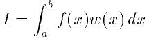
������
 �ϽŤߴؿ�(���̤�����ʬ�ؿ��Ǥ�
 )�Ǥ���. �桼�����ϼ�������������ꤹ�����и����ϰ�
(epsabs, epsrel)�����Ǥ���:
)�Ǥ���. �桼�����ϼ�������������ꤹ�����и����ϰ�
(epsabs, epsrel)�����Ǥ���:

������
 �ϥ��르�ꥺ��ˤ������줿����Ū����ͤǤ���. ���르�ꥺ������и���
 ����������ߤ�������ɾ������:

�롼����ϸ����ϰϤ���̩������ȼ�«���ʤ��ʤ�. ���ξ��������������
�ɤζ���ͤ��֤����.
QUADPACK�ˤ��륢�르�ꥺ��ϼ��Τ褦��̾���դ���§�˽��äƤ���:
Q - ���ѥ롼����
N - ��Ŭ��Ū��ʬ
A - Ŭ��Ū��ʬ
G - ������ʬ(�桼�������)
W - ����ʬ�ؿ��˽ŤߤŤ��ؿ�����
S - ȯ����ޤ���ʬ
P - �ð�����ޤ���ʬ
I - ̵���ϰϤǤ���ʬ
O - cos�ޤ���sin�ˤ�뿶ư�ؿ��ǤνŤߤŤ�
F - �ա��ꥨ��ʬ
C - ������������
���르�ꥺ��ˤ�, �⼡������㼡�ε�§�ˤ��1�Ф���ʬ§���Ȥ��Ƥ���.
�⼡��§�϶����ϰϤ���ʬ�ζ���ͤ������Τ˻Ȥ���. �⼡������㼡��
��̤κ��϶���θ���ɾ�����Ѥ�����.
���̤�(�ŤߤΤʤ�)�ؿ�����ʬ���르�ꥺ���Gauss-Kronrod§�˴�Ť��Ƥ���.
Gauss-Kronrod§��m���θ�ŵŪ��������ʬ����Ϥޤ�. �����
2m+1���ι⼡Kronrod§��Ϳ����褦�˲����������ղä���. Kornrod§
�ϥ�����§��ɾ�������ؿ��ͤ�����Ѥ���ΤǸ���Ū�Ǥ���. �⼡Kronrod§��
��ʬ�κ��ɶ���ͤȤ����Ѥ����, �����2�Ĥε�§�κ��϶�������Ȥ���ɾ��
�����.
�Ťߴؿ��Τ�������ʬ�ؿ��ξ���Clenshaw-Curtis����ˡ���Ѥ�����.
Clenshaw-Curtis§��n��Chebyschev¿�༰���������ʬ�ؿ���Ŭ�Ѥ���.
����¿�༰�ϸ�̩����ʬ�Ǥ���Τ�, ��������ʬ�ؿ�����ʬ����ͤ�������.
ChebyschevŸ���϶������ɤ��뤿��˹⼡�˳�ĥ���뤳�Ȥ��Ǥ���. ����ʬ��
�����ð���(��¾����ħ)��Chebyschev����Ǥϼ�«���٤�����. QUADPACK
�ǻȤ��Ƥ������Clenshaw-Curtis§�ϼ�«���٤����뤤���Ĥ������ѽŤߴ�
����ʬΥ���Ƥ���. �����νŤߴؿ���Chebyschev¿�༰���Ф����ѷ�
Chebyschev�⡼�����Ȥ��Ƥ��餫�������Ū����ʬ����Ƥ���. ���Υ⡼��
��Ȥȴؿ���Chebyschev������Ȥߤ��碌�뤳�Ȥˤ�깥������ʬ��¹ԤǤ���.
�ؿ����ð���ʬ�˲���Ū��ʬ��Ȥ����ȤǸ�̩���껦���뤳�Ȥ��Ǥ�, ��ʬ����
�μ�«���ʤ�����Ǥ���.
QNG���르�ꥺ���, �����87��������ʬ�ؿ��Υ���ץ��Ԥ�����
Gauss-Kronrod§�ˤ����Ŭ���ץ���������Ǥ���. ����ˤ���餫�ʴؿ���
��®����ʬ�Ǥ���.
- Function: int gsl_integration_qng (const gsl_function *f, double a, double b, double epsabs, double epsrel, double * result, double * abserr, size_t * neval)
-
���δؿ���, (a,b)���f����ʬ�ζ���ͤ��ᤵ������Ф����
���и���epsabs�����epsrel���ϰ���ˤ���¤�10��, 21��, 43��
�����87����Gauss-Kronrod��ʬ��¹Ԥ���. ���δؿ��Ϻǽ�Ū�ʶ����
result, ���и����θ��Ѥ�abserr, �Ѥ���줿�ؿ�ɾ����
neval���֤�. Gauss-Kronrod§��, �ؿ�ɾ���������餹����, ���ʤ�
���ʤη�̤����Ѥ���褦�߷פ���Ƥ���.
QAG���르�ꥺ��ϴ�ñ��Ŭ��Ū��ʬ�ץ���������Ǥ���. ��ʬ��֤�ʬ�䤷,
���ʤǺ��縫�Ѥ������Ϳ�����֤�ʬ�䤹��. ����ˤ�����Τθ���������,
��֤�ʬ�������ʬ�ؿ��ζɽ�Ū�����˽��椹�뤳�Ȥˤʤ�. ����ʬ���֤�
gsl_integration_workspace��¤�ΤǴ�������, ���, ���, ������ɾ��
��������Ǽ�����.
- Function: gsl_integration_workspace * gsl_integration_workspace_alloc (size_t n)
-
���δؿ���n�Ĥ������٤ζ��, ��ʬ���, ɾ���������Ǽ����Τ˽�ʬ
�ʺ�ȶ��֤���ݤ���.
- Function: void gsl_integration_workspace_free (gsl_integration_workspace * w)
-
���δؿ��Ϻ�ȶ���w�˳�ꤢ�Ƥ��Ƥ���������������.
- Function: int gsl_integration_qag (const gsl_function *f, double a, double b, double epsabs, double epsrel, size_t limit, int key, gsl_integration_workspace * workspace, double * result, double * abserr)
-
���δؿ���(a,b)���f����ʬ�ζ���ͤ��ᤵ������Ф������
�и���epsabs�����epsrel���ϰ���ˤ���¤�Ŭ��Ū����ʬ��¹�
����. ���δؿ��Ϻǽ�Ū�ʶ����result, ���и�����ɾ����abserr
���֤�. ��ʬ§��key���ͤˤ����ꤵ���. key�ϼ��Υ���ܥ�̾
��������:
GSL_INTEG_GAUSS15  (key = 1)
GSL_INTEG_GAUSS21  (key = 2)
GSL_INTEG_GAUSS31  (key = 3)
GSL_INTEG_GAUSS41  (key = 4)
GSL_INTEG_GAUSS51  (key = 5)
GSL_INTEG_GAUSS61  (key = 6)
�����15, 21, 31, 41, 51, 61��Gauss-Kronrod§����������. �⼡§�ϳ�餫
�ʴؿ��Ǥ�������٤��褯�ʤ�. �㼡§����Ϣ³�Τ褦�ʶɽ�Ū������ޤ�ؿ�
�ǻ��֤�����Ǥ���.
��ʬ�γ��ʤ�, Ŭ��Ū��ʬ���ȥ�ƥ��˽���ɾ������������ζ�֤�ʬ�䤹��.
���ʬ��Ȥ��η�̤�workspace�dz�ꤢ�Ƥ������˳�Ǽ�����.
���ʬ����κ����ͤ�limit��Ϳ������. ����ϳ�ꤢ�Ƥ�����ΰ��
��������ۤ��ƤϤʤ�ʤ�.
��ʬ��֤˲���ʬ���ð�����¸�ߤ����, Ŭ��Ū�롼����ζ��ʬ�䤬�ð�����
�ޤ��˽��椷�Ƥ��ޤ�. ʬ�䤵�줿��֤�������������Ȥ���ˤ����ʬ�ζ�
���ͤϸ¤�줿���Ǥ�����«���ʤ�. ���μ�«���ޤˤ���®������. QAGS��
�르�ꥺ���Ŭ��Ū���ʬ���Wynn�ť��르�ꥺ���ͻ�礵��, �͡��ʲ���ʬ��
��������ʬ�ԡ��ɥ��åפ�����.
- Function: int gsl_integration_qags (const gsl_function * f, double a, double b, double epsabs, double epsrel, size_t limit, gsl_integration_workspace * workspace, double *result, double *abserr)
-
���δؿ���(a,b)���f����ʬ�ζ���ͤ��ᤵ������Ф������
�и���epsabs�����epsrel���ϰ���ˤ���¤�21��Gauss-Kronrod
��ʬ§��Ŭ��Ū�˼¹Ԥ���. ��̤�
 ���르�ꥺ��ˤ�곰�ޤ���, ��Ϣ³�����ʬ�ð�����¸�ߤ�����ʬ�μ�«���
®������. ���δؿ��ϳ��ޤˤ��ǽ������result, ���и�����ɾ����
abserr���֤�. ���ʬ��Ȥ��η�̤�workspace�dz�ꤢ�Ƥ���
����˳�Ǽ�����. ʬ���֤κ������limit�ǻ��ꤹ��. ��ȶ��֤�
��ꤢ�ƥ�������ۤ��ƤϤʤ�ʤ�.
���르�ꥺ��ˤ�곰�ޤ���, ��Ϣ³�����ʬ�ð�����¸�ߤ�����ʬ�μ�«���
®������. ���δؿ��ϳ��ޤˤ��ǽ������result, ���и�����ɾ����
abserr���֤�. ���ʬ��Ȥ��η�̤�workspace�dz�ꤢ�Ƥ���
����˳�Ǽ�����. ʬ���֤κ������limit�ǻ��ꤹ��. ��ȶ��֤�
��ꤢ�ƥ�������ۤ��ƤϤʤ�ʤ�.
- Function: int gsl_integration_qagp (const gsl_function * f, double *pts, size_t npts, double epsabs, double epsrel, size_t limit, gsl_integration_workspace * workspace, double *result, double *abserr)
-
���δؿ��ϥ桼�����������ð����ξ����θ���ʤ���Ŭ��Ū����ʬ��¹�
���륢�르�ꥺ��QAGS�μ����Ǥ���. Ĺ��npts������pts�ˤ���ʬ
��֤�ü�����ð����ΰ��֤��Ǽ����. �㤨��, ���(a,b)���,
 ���ð���������ʬ��¹Ԥ�����(������
 ), ���Τ褦��pts�����Ϳ����:
pts[0] = a
pts[1] = x_1
pts[2] = x_2
pts[3] = x_3
pts[4] = b
������ npts = 5.
��ʬ��֤Ǥ��ð����ΰ��֤��ΤäƤ������, ���Υ롼����Τۤ���
QAGS����ᤤ.
- Function: int gsl_integration_qagi (gsl_function * f, double epsabs, double epsrel, size_t limit, gsl_integration_workspace * workspace, double *result, double *abserr)
-
���δؿ�����ͭ�����
 �Ǵؿ�f����ʬ����. ��ʬ���ѿ��Ѵ�
 �ˤ����
 �˼��������:

������QAGS���르�ꥺ����Ѥ�����ʬ�����. �ѿ��Ѵ��ˤ�긶���˲���ʬ����
�������Ǥ��Ƥ��ޤ��Τ�, �̾��QAGS��21��Gauss-Kronrod§��15��§�ˤ�����
����. ���ξ���㼡§�Τۤ���������Ū������Ǥ���.
- Function: int gsl_integration_qagiu (gsl_function * f, double a, double epsabs, double epsrel, size_t limit, gsl_integration_workspace * workspace, double *result, double *abserr)
-
���δؿ���Ⱦ��ͭ�����
 ��Ǵؿ�f����ʬ����. ��ʬ���ѿ��Ѵ�
 �ˤ����
�˼��������.
�ˤ����
�˼��������.
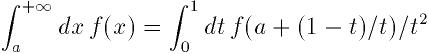
������QAGS���르�ꥺ����Ѥ�����ʬ�����.
- Function: int gsl_integration_qagil (gsl_function * f, double b, double epsabs, double epsrel, size_t limit, gsl_integration_workspace * workspace, double *result, double *abserr)
-
���δؿ���Ⱦ��ͭ�����
 ��Ǵؿ�f����ʬ����. ��ʬ���ѿ��Ѵ�
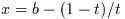 �ˤ����
�˼��������.
�ˤ����
�˼��������.
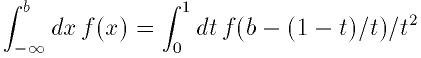
������QAGS���르�ꥺ����Ѥ�����ʬ�����.
- Function: int gsl_integration_qawc (gsl_function *f, double a, double b, double c, double epsabs, double epsrel, size_t limit, gsl_integration_workspace * workspace, double * result, double * abserr)
-
���δؿ���
 ���f����ʬ��c�Ǥ��ð����Υ����������ͤ����.
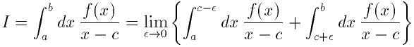
QAG��Ŭ��Ūʬ�䥢�르�ꥺ�ब�Ȥ��뤬, �ð���
 ��ʬ�䤵��ʤ��褦�˹��פ���Ƥ���. ʬ���֤���
��ޤ�Ǥ�����, �������˶ᤤ�������̤�25���ѷ�Clenshaw-Curtis§���ð�
�����뤿��˻Ȥ���. �ð�������Υ�줿���Ǥ��̾��15��
Gauss-Kronrod��ʬ§���Ȥ���.
��ʬ�䤵��ʤ��褦�˹��פ���Ƥ���. ʬ���֤���
��ޤ�Ǥ�����, �������˶ᤤ�������̤�25���ѷ�Clenshaw-Curtis§���ð�
�����뤿��˻Ȥ���. �ð�������Υ�줿���Ǥ��̾��15��
Gauss-Kronrod��ʬ§���Ȥ���.
QAWS���르�ꥺ���, ����ʬ�ؿ�����ʬ�ΰ��ü�����п�Ū��ȯ����Ȥ���
�Ѥ�����. ����Ū�˷����뤿��, Chebyschev�⡼���Ȥ餫�������
�Ƥ���.
- Function: gsl_integration_qaws_table * gsl_integration_qaws_table_alloc (double alpha, double beta, int mu, int nu)
-
���δؿ���gsl_integration_gaws_table���ΰ����ݤ�, �ð����νŤ�
�ؿ�
 ��ѥ���
 ��ɽ�����뤿��κ���ΰ���ꤢ�Ƥ�:

������
 �Ǥ���. �Ťߴؿ���
 ,
,  ���ͤˤ��ʲ���4�Ĥη���Ȥ�:
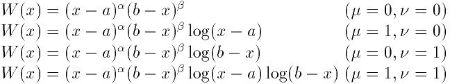
��
����ʬ���������ޤ����ꤵ��ʤ��Ƥ�褤. ��������ʬ�ΰ��ü���Ǥ���.
���δؿ���, ���顼�����Ф���ʤ����, ��������ꤢ�Ƥ�줿
gsl_integration_qaws_table�ؤΥݥ����֤�. ���顼�ξ��ˤ�0��
�֤�.
- Function: int gsl_integration_qaws_table_set (gsl_integration_qaws_table * t, double alpha, double beta, int mu, int nu)
-
���δؿ���
gsl_integration_qaws_table��¤��t�Υѥ���
���ѹ�����.
- Function: void gsl_integration_qaws_table_free (gsl_integration_qaws_table * t)
-
���δؿ���
gsl_integration_qaws_table��¤��t�˳�ꤢ�Ƥ�줿
������������.
- Function: int gsl_integration_qaws (gsl_function * f, const double a, const double b, gsl_integration_qaws_table * t, const double epsabs, const double epsrel, const size_t limit, gsl_integration_workspace * workspace, double *result, double *abserr)
-
���δؿ����ð����Ťߴؿ�
 ���Ѥ��ƶ��
��Ǵؿ�f(x)����ʬ����. �ѥ���
�ϥơ��֥�t�����������.
���Ѥ��ƶ��
��Ǵؿ�f(x)����ʬ����. �ѥ���
�ϥơ��֥�t�����������.

QAG��Ŭ��Ūʬ�䥢�르�ꥺ�ब�Ѥ�����. ʬ���֤�ü�����ޤޤ��Ȥ���
�ü�25���ѷ�Clenshaw-Curtis§���ð������뤿����Ѥ�����. ü�����
�ޤʤ���֤Ǥ��̾��15��Gauss-Kronrod§���Ѥ�����.
QAWO���르�ꥺ��Ͽ�ư����
 ������ʬ�������. ����Ū�˷����뤿��, ���ΰ��Ҥ餫���������
Chebyschev�⡼���ȤΥơ��֥뤬ɬ�פȤʤ�.
������ʬ�������. ����Ū�˷����뤿��, ���ΰ��Ҥ餫���������
Chebyschev�⡼���ȤΥơ��֥뤬ɬ�פȤʤ�.
- Function: gsl_integration_qawo_table * gsl_integration_qawo_table_alloc (double omega, double L, enum gsl_integration_qawo_enum sine, size_t n)
-
���δؿ���gsl_integration_qawo_table��¤�ΤΤ���˶��֤��ꤢ��,
�ѥ���
 ���ĥ�����ޤ��ϥ�������νŤߴؿ�
�Τ���κ���ΰ�Ȥʤ�.
���ĥ�����ޤ��ϥ�������νŤߴؿ�
�Τ���κ���ΰ�Ȥʤ�.
�ѥ���L�ϴؿ�����ʬ�ΰ��Ĺ��
 ��Ϳ����. �����������������ϥѥ���sine�ǹԤ���. �ͤˤ�
�ʲ��Υ���ܥ��ͤ��Ѥ���:
��Ϳ����. �����������������ϥѥ���sine�ǹԤ���. �ͤˤ�
�ʲ��Υ���ܥ��ͤ��Ѥ���:
GSL_INTEG_COSINE
GSL_INTEG_SINE
gsl_integration_qawo_table����ʬ������ɬ�פȤʤ뻰�Ѵؿ�ɽ�Ǥ���.
�ѥ���n�ˤ�������뷸���Υ�٥뤬���ꤵ���. �ƥ�٥�ϴ�
��L��ʬ�����������Τ�, n��٥��Ĺ��
 �ޤǤ�ʬ���֤��б��Ǥ���. ��ʬ�롼����
gsl_integration_qawo��,
�ᤵ�줿���٤��Ф��ƥ�٥���������Ƥ�����ˤ�GSL_ETABLE��
�֤�.
- Function: int gsl_integration_qawo_table_set (gsl_integration_qawo_table * t, double omega, double L, enum gsl_integration_qawo_enum sine)
-
���δؿ���¸�ߤ������ΰ�t�Υѥ���omega, L,
sine���ѹ�����.
- Function: int gsl_integration_qawo_table_set_length (gsl_integration_qawo_table * t, double L)
-
���δؿ��Ϻ���ΰ�t��Ĺ���Υѥ���L���ѹ�����.
- Function: void gsl_integration_qawo_table_free (gsl_integration_qawo_table * t)
-
���δؿ��Ϻ���ΰ�t�˳�ꤢ�Ƥ�줿������������.
- Function: int gsl_integration_qawo (gsl_function * f, const double a, const double epsabs, const double epsrel, const size_t limit, gsl_integration_workspace * workspace, gsl_integration_qawo_table * wf, double *result, double *abserr)
-
���δؿ���, �ơ��֥�wf����������Ťߴؿ�
���Ѥ�, ���
��Ǵؿ�f����ʬ�������Ŭ��Ū���르�ꥺ��Ǥ���.
��ʬ�μ�«��®���뤿��, ��̤�
���르�ꥺ����Ѥ��Ƴ��ޤ����. �ؿ��Ϻǽ�Ū�ʿ�����result, ���и�
����ɾ����abserr���֤�. ʬ���֤Ȥ��η�̤�workspace�Υ��
��˳�Ǽ�����. ʬ���֤κ������limit��Ϳ������. ����Ϻ����
��γ�ꤢ�ƥ�������ۤ��ƤϤʤ�ʤ�.
���礭�ʡ���
 ����ʬ���֤�25��Clenshaw-Curtis��ʬ§���Ѥ��Ʒ���, ��ư���������.
�־����ʡ���
����ʬ���֤�25��Clenshaw-Curtis��ʬ§���Ѥ��Ʒ���, ��ư���������.
�־����ʡ���
 ����ʬ���֤Ǥ�15��Gauss-Kronrod��ʬ���Ѥ���.
- Function: int gsl_integration_qawf (gsl_function * f, const double a, const double epsabs, const size_t limit, gsl_integration_workspace * workspace, gsl_integration_workspace * cycle_workspace, gsl_integration_qawo_table * wf, double *result, double *abserr)
-
���δؿ���Ⱦ��ͭ�����
 �Ǥδؿ�f��Fourier��ʬ�������.
�ѥ���
 �ϥơ��֥�wf(Ĺ��L�Ϲ������ͤ�Ȥ뤳�Ȥ��Ǥ���. Fourier��ʬ
��Ŭ�ڤ��ͤȤʤ�褦�ˤ��δؿ��ˤ�ꥪ���С��饤�ɤ���뤫��Ǥ���)����
�Ȥ���. ��ʬ��QAWO���르�ꥺ���ȤäƳ�ʬ���֤Ƿ������.
�ϥơ��֥�wf(Ĺ��L�Ϲ������ͤ�Ȥ뤳�Ȥ��Ǥ���. Fourier��ʬ
��Ŭ�ڤ��ͤȤʤ�褦�ˤ��δؿ��ˤ�ꥪ���С��饤�ɤ���뤫��Ǥ���)����
�Ȥ���. ��ʬ��QAWO���르�ꥺ���ȤäƳ�ʬ���֤Ƿ������.
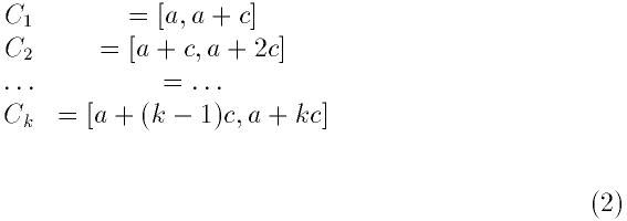
������
 �ϼ����δ���ܤС�����褦�����Ф��. �ƶ�֤���δ�Ϳ����椬���夷,
f������ñĴ����������ˤ�ñĴ��������. ���ο�����¤�
���르�ꥺ��Dz�®����.
�ϼ����δ���ܤС�����褦�����Ф��. �ƶ�֤���δ�Ϳ����椬���夷,
f������ñĴ����������ˤ�ñĴ��������. ���ο�����¤�
���르�ꥺ��Dz�®����.
���δؿ������Τ����и���abserr�Dz���������. �ʲ��Υ��ȥ�ƥ�����
������: �ƶ��
 �ǥ��르�ꥺ��ϵ��Ƹ�����ã�����褦�Ȥ���:
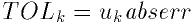
������
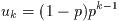 �����
�����
 �Ǥ���. �ƶ�֤λ��Ѵؿ���δ�Ϳ���¤����Τε��Ƹ���abserr��Ϳ����.
ʬ���֤���ʬ�˺���ȯ����������ʬ���֤��Ф������������¤���.
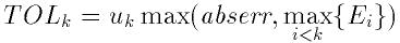
������
 �϶��
�Ǥ�ɾ�������Ǥ���.
�϶��
�Ǥ�ɾ�������Ǥ���.
ʬ���֤Ȥ��η�̤�workspace�Υ���˳�Ǽ�����. ʬ���֤κ���
����limit��Ϳ������. ����ΰ�γ�ꤢ�ƥ���������礭���ʤ��Ƥ�
�ʤ�ʤ�. ��ʬ���֤Ǥ���ʬ�ˤ�cycle_workspace�Υ��꤬QAWO����
���ꥺ��Τ���κ���ΰ�Ȥ����Ѥ�����.
���������˴ؤ���ɸ�२�顼�����ɤ�¾, �����δؿ��ϼ����ͤ��֤�:
GSL_EMAXITER
-
���ʬ��κ������ۤ���.
GSL_EROUND
-
�Ǥ���������ˤ������ϰϤ��Ϥ��ʤ��ä�, �⤷���ϳ��ޥơ��֥���Ǥ�����
���������Ф��줿.
GSL_ESING
-
����ʬ�Ǥʤ��ð����⤷���Ϥ���¾������ʬ�ؿ��ΰ���������ʬ�����˸�
�Ĥ��ä�.
GSL_EDIVERGE
-
��ʬ��ȯ������, �⤷������ʬ�μ�«���٤�����.
��ʬ�롼����QAGS��ͭ����ʬ���礯�Υ��饹�Ƿ��Ǥ���. �㤨��, ��
�Τ褦����ʬ��ͤ���. ����ϸ������п�Ū���ð�������:
�ʲ��Υץ������Ϥ�����ʬ�����и���1e-7����ʬ�����ΤǤ���.
#include <stdio.h>
#include <math.h>
#include <gsl/gsl_integration.h>
double f (double x, void * params) {
double alpha = *(double *) params;
double f = log(alpha*x) / sqrt(x);
return f;
}
int
main (void)
{
gsl_integration_workspace * w
= gsl_integration_workspace_alloc(1000);
double result, error;
double expected = -4.0;
double alpha = 1.0;
gsl_function F;
F.function = &f;
F.params = α
gsl_integration_qags (&F, 0, 1, 0, 1e-7, 1000,
w, &result, &error);
printf("result = % .18f\n", result);
printf("exact result = % .18f\n", expected);
printf("estimated error = % .18f\n", error);
printf("actual error = % .18f\n", result - expected);
printf("intervals = %d\n", w->size);
return 0;
}
�ʲ��˼�����̤�, 8��ʬ�䤹�뤳�Ȥˤ��˾������٤�ã���Ǥ������Ȥ�
�Ƥ���.
bash$ ./a.out
result          = -3.999999999999973799
exact result    = -4.000000000000000000
estimated error =  0.000000000000246025
actual error    =  0.000000000000026201
intervals =  8
�º�, QAGS���Ѥ����볰�ޥץ���������������٤��ܶᤤ���٤��
��. ���ޥץ�����������֤�ɾ�������ϼºݤθ��������礭��. �����Τ���1
��Υޡ������ȤäƤ��뤫��Ǥ���.
�ʲ����ܤ�QUADPACK�λ��ͽ�η����ǤǤ���, ��Ԥˤ��줿��Τ�
����. ���르�ꥺ��, �ץ���������, �ƥ��ȥץ������, ���������꤬�ܤ���
��Ƥ���. ������ʬ�˴ؤ���ͭ�Ѥʥ��ɥХ�����, QUADPACK�γ�ȯ���Ѥ�
��줿������ʬ�˴ؤ��뻲�ͽ��ܤ���Ƥ���.
-
R. Piessens, E. de Doncker-Kapenga, C.W. Uberhuber, D.K. Kahaner.
QUADPACK A subroutine package for automatic integration
Springer Verlag, 1983.
The library provides a large collection of random number generators
which can be accessed through a uniform interface. Environment
variables allow you to select different generators and seeds at runtime,
so that you can easily switch between generators without needing to
recompile your program. Each instance of a generator keeps track of its
own state, allowing the generators to be used in multi-threaded
programs. Additional functions are available for transforming uniform
random numbers into samples from continuous or discrete probability
distributions such as the Gaussian, log-normal or Poisson distributions.
These functions are declared in the header file `gsl_rng.h'.
In 1988, Park and Miller wrote a paper entitled "Random number
generators: good ones are hard to find." [Commun. ACM, 31, 1192--1201].
Fortunately, some excellent random number generators are available,
though poor ones are still in common use. You may be happy with the
system-supplied random number generator on your computer, but you should
be aware that as computers get faster, requirements on random number
generators increase. Nowadays, a simulation that calls a random number
generator millions of times can often finish before you can make it down
the hall to the coffee machine and back.
A very nice review of random number generators was written by Pierre
L'Ecuyer, as Chapter 4 of the book: Handbook on Simulation, Jerry Banks,
ed. (Wiley, 1997). The chapter is available in postscript from from
L'Ecuyer's ftp site (see references). Knuth's volume on Seminumerical
Algorithms (originally published in 1968) devotes 170 pages to random
number generators, and has recently been updated in its 3rd edition
(1997).
It is brilliant, a classic. If you don't own it, you should stop reading
right now, run to the nearest bookstore, and buy it.
A good random number generator will satisfy both theoretical and
statistical properties. Theoretical properties are often hard to obtain
(they require real math!), but one prefers a random number generator
with a long period, low serial correlation, and a tendency not to
"fall mainly on the planes." Statistical tests are performed with
numerical simulations. Generally, a random number generator is used to
estimate some quantity for which the theory of probability provides an
exact answer. Comparison to this exact answer provides a measure of
"randomness".
It is important to remember that a random number generator is not a
"real" function like sine or cosine. Unlike real functions, successive
calls to a random number generator yield different return values. Of
course that is just what you want for a random number generator, but to
achieve this effect, the generator must keep track of some kind of
"state" variable. Sometimes this state is just an integer (sometimes
just the value of the previously generated random number), but often it
is more complicated than that and may involve a whole array of numbers,
possibly with some indices thrown in. To use the random number
generators, you do not need to know the details of what comprises the
state, and besides that varies from algorithm to algorithm.
The random number generator library uses two special structs,
gsl_rng_type which holds static information about each type of
generator and gsl_rng which describes an instance of a generator
created from a given gsl_rng_type.
The functions described in this section are declared in the header file
`gsl_rng.h'.
- Random: gsl_rng * gsl_rng_alloc (const gsl_rng_type * T)
-
This function returns a pointer to a newly-created
instance of a random number generator of type T.
For example, the following code creates an instance of the Tausworthe
generator,
gsl_rng * r = gsl_rng_alloc (gsl_rng_taus);
If there is insufficient memory to create the generator then the
function returns a null pointer and the error handler is invoked with an
error code of GSL_ENOMEM.
The generator is automatically initialized with the default seed,
gsl_rng_default_seed. This is zero by default but can be changed
either directly or by using the environment variable GSL_RNG_SEED
(see section Random number environment variables).
The details of the available generator types are
described later in this chapter.
- Random: void gsl_rng_set (const gsl_rng * r, unsigned long int s)
-
This function initializes (or `seeds') the random number generator. If
the generator is seeded with the same value of s on two different
runs, the same stream of random numbers will be generated by successive
calls to the routines below. If different values of s are
supplied, then the generated streams of random numbers should be
completely different. If the seed s is zero then the standard seed
from the original implementation is used instead. For example, the
original Fortran source code for the
ranlux generator used a seed
of 314159265, and so choosing s equal to zero reproduces this when
using gsl_rng_ranlux.
- Random: void gsl_rng_free (gsl_rng * r)
-
This function frees all the memory associated with the generator
r.
The following functions return uniformly distributed random numbers,
either as integers or double precision floating point numbers. To obtain
non-uniform distributions see section Random Number Distributions.
- Random: unsigned long int gsl_rng_get (const gsl_rng * r)
-
This function returns a random integer from the generator r. The
minimum and maximum values depend on the algorithm used, but all
integers in the range [min,max] are equally likely. The
values of min and max can determined using the auxiliary
functions
gsl_rng_max (r) and gsl_rng_min (r).
- Random: double gsl_rng_uniform (const gsl_rng * r)
-
This function returns a double precision floating point number uniformly
distributed in the range [0,1). The range includes 0.0 but excludes 1.0.
The value is typically obtained by dividing the result of
gsl_rng_get(r) by gsl_rng_max(r) + 1.0 in double
precision. Some generators compute this ratio internally so that they
can provide floating point numbers with more than 32 bits of randomness
(the maximum number of bits that can be portably represented in a single
unsigned long int).
- Random: double gsl_rng_uniform_pos (const gsl_rng * r)
-
This function returns a positive double precision floating point number
uniformly distributed in the range (0,1), excluding both 0.0 and 1.0.
The number is obtained by sampling the generator with the algorithm of
gsl_rng_uniform until a non-zero value is obtained. You can use
this function if you need to avoid a singularity at 0.0.
- Random: unsigned long int gsl_rng_uniform_int (const gsl_rng * r, unsigned long int n)
-
This function returns a random integer from 0 to n-1 inclusive.
All integers in the range [0,n-1] are equally likely, regardless
of the generator used. An offset correction is applied so that zero is
always returned with the correct probability, for any minimum value of
the underlying generator.
If n is larger than the range of the generator then the function
calls the error handler with an error code of GSL_EINVAL and
returns zero.
The following functions provide information about an existing
generator. You should use them in preference to hard-coding the generator
parameters into your own code.
- Random: const char * gsl_rng_name (const gsl_rng * r)
-
This function returns a pointer to the name of the generator.
For example,
printf("r is a '%s' generator\n",
       gsl_rng_name (r));
would print something like r is a 'taus' generator.
- Random: unsigned long int gsl_rng_max (const gsl_rng * r)
-
gsl_rng_max returns the largest value that gsl_rng_get
can return.
- Random: unsigned long int gsl_rng_min (const gsl_rng * r)
-
gsl_rng_min returns the smallest value that gsl_rng_get
can return. Usually this value is zero. There are some generators with
algorithms that cannot return zero, and for these generators the minimum
value is 1.
- Random: void * gsl_rng_state (const gsl_rng * r)
-
- Random: size_t gsl_rng_size (const gsl_rng * r)
-
These function return a pointer to the state of generator r and
its size. You can use this information to access the state directly. For
example, the following code will write the state of a generator to a
stream,
void * state = gsl_rng_state (r);
size_t n = gsl_rng_size (r);
fwrite (state, n, 1, stream);
- Random: const gsl_rng_type ** gsl_rng_types_setup (void)
-
This function returns a pointer to an array of all the available
generator types, terminated by a null pointer. The function should be
called once at the start of the program, if needed. The following code
fragment shows how to iterate over the array of generator types to print
the names of the available algorithms,
const gsl_rng_type **t, **t0;

t0 = gsl_rng_types_setup ();

printf("Available generators:\n");

for (t = t0; *t != 0; t++)
  {
    printf("%s\n", (*t)->name);
  }
The library allows you to choose a default generator and seed from the
environment variables GSL_RNG_TYPE and GSL_RNG_SEED and
the function gsl_rng_env_setup. This makes it easy try out
different generators and seeds without having to recompile your program.
- Function: const gsl_rng_type * gsl_rng_env_setup (void)
-
This function reads the environment variables
GSL_RNG_TYPE and
GSL_RNG_SEED and uses their values to set the corresponding
library variables gsl_rng_default and
gsl_rng_default_seed. These global variables are defined as
follows,
extern const gsl_rng_type *gsl_rng_default
extern unsigned long int gsl_rng_default_seed
The environment variable GSL_RNG_TYPE should be the name of a
generator, such as taus or mt19937. The environment
variable GSL_RNG_SEED should contain the desired seed value. It
is converted to an unsigned long int using the C library function
strtoul.
If you don't specify a generator for GSL_RNG_TYPE then
gsl_rng_mt19937 is used as the default. The initial value of
gsl_rng_default_seed is zero.
Here is a short program which shows how to create a global
generator using the environment variables GSL_RNG_TYPE and
GSL_RNG_SEED,
#include <stdio.h>
#include <gsl/gsl_rng.h>

gsl_rng * r;  /* global generator */

int
main (void)
{
  const gsl_rng_type * T;

  gsl_rng_env_setup();

  T = gsl_rng_default;
  r = gsl_rng_alloc (T);

  printf("generator type: %s\n", gsl_rng_name (r));
  printf("seed = %u\n", gsl_rng_default_seed);
  printf("first value = %u\n", gsl_rng_get (r));
  return 0;
}
Running the program without any environment variables uses the initial
defaults, an mt19937 generator with a seed of 0,
bash$ ./a.out
generator type: mt19937
seed = 0
first value = 2867219139
By setting the two variables on the command line we can
change the default generator and the seed,
bash$ GSL_RNG_TYPE="taus" GSL_RNG_SEED=123 ./a.out
GSL_RNG_TYPE=taus
GSL_RNG_SEED=123
generator type: taus
seed = 123
first value = 2720986350
The above methods ignore the random number `state' which changes from
call to call. It is often useful to be able to save and restore the
state. To permit these practices, a few somewhat more advanced
functions are supplied. These include:
- Random: int gsl_rng_memcpy (gsl_rng * dest, const gsl_rng * src)
-
This function copies the random number generator src into the
pre-existing generator dest, making dest into an exact copy
of src. The two generators must be of the same type.
- Random: gsl_rng * gsl_rng_clone (const gsl_rng * r)
-
This function returns a pointer to a newly created generator which is an
exact copy of the generator r.
- Random: void gsl_rng_print_state (const gsl_rng * r)
-
This function prints a hex-dump of the state of the generator r to
stdout. At the moment its only use is for debugging.
The functions described above make no reference to the actual algorithm
used. This is deliberate so that you can switch algorithms without
having to change any of your application source code. The library
provides a large number of generators of different types, including
simulation quality generators, generators provided for compatibility
with other libraries and historical generators from the past.
The following generators are recommended for use in simulation. They
have extremely long periods, low correlation and pass most statistical
tests.
- Generator: gsl_rng_mt19937
-
The MT19937 generator of Makoto Matsumoto and Takuji Nishimura is a
variant of the twisted generalized feedback shift-register algorithm,
and is known as the "Mersenne Twister" generator. It has a Mersenne
prime period of
2^19937 - 1 (about
10^6000) and is
equi-distributed in 623 dimensions. It has passed the DIEHARD
statistical tests. It uses 624 words of state per generator and is
comparable in speed to the other generators. The original generator used
a default seed of 4357 and choosing s equal to zero in
gsl_rng_set reproduces this.
For more information see,
-
Makoto Matsumoto and Takuji Nishimura, "Mersenne Twister: A
623-dimensionally equidistributed uniform pseudorandom number
generator". ACM Transactions on Modeling and Computer
Simulation, Vol. 8, No. 1 (Jan. 1998), Pages 3-30
The generator gsl_rng_19937 uses the corrected version of the
seeding procedure published later by the two authors above. The
original seeding procedure suffered from low-order periodicity, but can
be used by selecting the alternate generator gsl_rng_mt19937_1998.
- Generator: gsl_rng_ranlxs0
-
- Generator: gsl_rng_ranlxs1
-
- Generator: gsl_rng_ranlxs2
-
The generator ranlxs0 is a second-generation version of the
RANLUX algorithm of L@"uscher, which produces "luxury random
numbers". This generator provides single precision output (24 bits) at
three luxury levels ranlxs0, ranlxs1 and ranlxs2.
It uses double-precision floating point arithmetic internally and can be
significantly faster than the integer version of ranlux,
particularly on 64-bit architectures. The period of the generator is
about @c{$10^{171}$}
10^171. The algorithm has mathematically proven properties and
can provide truly decorrelated numbers at a known level of randomness.
The higher luxury levels provide additional decorrelation between samples
as an additional safety margin.
- Generator: gsl_rng_ranlxd1
-
- Generator: gsl_rng_ranlxd2
-
These generators produce double precision output (48 bits) from the
RANLXS generator. The library provides two luxury levels
ranlxd1 and ranlxd2.
- Generator: gsl_rng_ranlux
-
- Generator: gsl_rng_ranlux389
-
The ranlux generator is an implementation of the original
algorithm developed by L@"uscher. It uses a
lagged-fibonacci-with-skipping algorithm to produce "luxury random
numbers". It is a 24-bit generator, originally designed for
single-precision IEEE floating point numbers. This implementation is
based on integer arithmetic, while the second-generation versions
RANLXS and RANLXD described above provide floating-point
implementations which will be faster on many platforms.
The period of the generator is about @c{$10^{171}$}
10^171. The algorithm has mathematically proven properties and
it can provide truly decorrelated numbers at a known level of
randomness. The default level of decorrelation recommended by L@"uscher
is provided by gsl_rng_ranlux, while gsl_rng_ranlux389
gives the highest level of randomness, with all 24 bits decorrelated.
Both types of generator use 24 words of state per generator.
For more information see,
-
M. L@"uscher, "A portable high-quality random number generator for
lattice field theory calculations", Computer Physics
Communications, 79 (1994) 100-110.
-
F. James, "RANLUX: A Fortran implementation of the high-quality
pseudo-random number generator of L@"uscher", Computer Physics
Communications, 79 (1994) 111-114
- Generator: gsl_rng_cmrg
-
This is a combined multiple recursive generator by L'Ecuyer.
Its sequence is,
where the two underlying generators x_n and y_n are,
with coefficients
a_1 = 0,
a_2 = 63308,
a_3 = -183326,
b_1 = 86098,
b_2 = 0,
b_3 = -539608,
and moduli
m_1 = 2^31 - 1 = 2147483647
and
m_2 = 2145483479.
The period of this generator is
2^205
(about
10^61). It uses
6 words of state per generator. For more information see,
-
P. L'Ecuyer, "Combined Multiple Recursive Random Number
Generators," Operations Research, 44, 5 (1996), 816--822.
- Generator: gsl_rng_mrg
-
This is a fifth-order multiple recursive generator by L'Ecuyer, Blouin
and Coutre. Its sequence is,
with
a_1 = 107374182,
a_2 = a_3 = a_4 = 0,
a_5 = 104480
and
m = 2^31 - 1.
The period of this generator is about
10^46. It uses 5 words
of state per generator. More information can be found in the following
paper,
-
P. L'Ecuyer, F. Blouin, and R. Coutre, "A search for good multiple
recursive random number generators", ACM Transactions on Modeling and
Computer Simulation 3, 87-98 (1993).
- Generator: gsl_rng_taus
-
This is a maximally equidistributed combined Tausworthe generator by
L'Ecuyer. The sequence is,
where,
computed modulo
2^32. In the formulas above
^^
denotes "exclusive-or". Note that the algorithm relies on the properties
of 32-bit unsigned integers and has been implemented using a bitmask
of 0xFFFFFFFF to make it work on 64 bit machines.
The period of this generator is @c{$2^{88}$}
2^88 (about
10^26). It uses 3 words of state per generator. For more
information see,
-
P. L'Ecuyer, "Maximally Equidistributed Combined Tausworthe
Generators", Mathematics of Computation, 65, 213 (1996), 203--213.
- Generator: gsl_rng_gfsr4
-
The
gfsr4 generator is like a lagged-fibonacci generator, and
produces each number as an xor'd sum of four previous values.
Ziff (ref below) notes that "it is now widely known" that two-tap
registers (such as R250, which is described below)
have serious flaws, the most obvious one being the three-point
correlation that comes from the definition of the generator. Nice
mathematical properties can be derived for GFSR's, and numerics bears
out the claim that 4-tap GFSR's with appropriately chosen offsets are as
random as can be measured, using the author's test.
This implementation uses the values suggested the the example on p392 of
Ziff's article: A=471, B=1586, C=6988, D=9689.
If the offsets are appropriately chosen (such the one ones in
this implementation), then the sequence is said to be maximal.
I'm not sure what that means, but I would guess that means all
states are part of the same cycle, which would mean that the
period for this generator is astronomical; it is
(2^K)^D \approx 10^{93334}
where K=32 is the number of bits in the word, and D is the longest
lag. This would also mean that any one random number could
easily be zero; ie
0 <= r < 2^32.
Ziff doesn't say so, but it seems to me that the bits are
completely independent here, so one could use this as an efficient
bit generator; each number supplying 32 random bits. The quality of the
generated bits depends on the underlying seeding procedure, which
may need to be improved in some circumstances.
For more information see,
-
Robert M. Ziff, "Four-tap shift-register-sequence random-number
generators", Computers in Physics, 12(4), Jul/Aug
1998, pp 385-392.
The standard Unix random number generators rand, random
and rand48 are provided as part of GSL. Although these
generators are widely available individually often they aren't all
available on the same platform. This makes it difficult to write
portable code using them and so we have included the complete set of
Unix generators in GSL for convenience. Note that these generators
don't produce high-quality randomness and aren't suitable for work
requiring accurate statistics. However, if you won't be measuring
statistical quantities and just want to introduce some variation into
your program then these generators are quite acceptable.
- Generator: gsl_rng_rand
-
This is the BSD
rand() generator. Its sequence is
with
a = 1103515245,
c = 12345 and
m = 2^31.
The seed specifies the initial value,
x_1. The period of this
generator is
2^31, and it uses 1 word of storage per
generator.
- Generator: gsl_rng_random_bsd
-
- Generator: gsl_rng_random_libc5
-
- Generator: gsl_rng_random_glibc2
-
These generators implement the
random() family of functions, a
set of linear feedback shift register generators originally used in BSD
Unix. There are several versions of random() in use today: the
original BSD version (e.g. on SunOS4), a libc5 version (found on
older GNU/Linux systems) and a glibc2 version. Each version uses a
different seeding procedure, and thus produces different sequences.
The original BSD routines accepted a variable length buffer for the
generator state, with longer buffers providing higher-quality
randomness. The random() function implemented algorithms for
buffer lengths of 8, 32, 64, 128 and 256 bytes, and the algorithm with
the largest length that would fit into the user-supplied buffer was
used. To support these algorithms additional generators are available
with the following names,
gsl_rng_random8_bsd
gsl_rng_random32_bsd
gsl_rng_random64_bsd
gsl_rng_random128_bsd
gsl_rng_random256_bsd
where the numeric suffix indicates the buffer length. The original BSD
random function used a 128-byte default buffer and so
gsl_rng_random_bsd has been made equivalent to
gsl_rng_random128_bsd. Corresponding versions of the libc5
and glibc2 generators are also available, with the names
gsl_rng_random8_libc5, gsl_rng_random8_glibc2, etc.
- Generator: gsl_rng_rand48
-
This is the Unix
rand48 generator. Its sequence is
defined on 48-bit unsigned integers with
a = 25214903917,
c = 11 and
m = 2^48.
The seed specifies the upper 32 bits of the initial value, x_1,
with the lower 16 bits set to 0x330E. The function
gsl_rng_get returns the upper 32 bits from each term of the
sequence. This does not have a direct parallel in the original
rand48 functions, but forcing the result to type long int
reproduces the output of mrand48. The function
gsl_rng_uniform uses the full 48 bits of internal state to return
the double precision number x_n/m, which is equivalent to the
function drand48. Note that some versions of the GNU C Library
contained a bug in mrand48 function which caused it to produce
different results (only the lower 16-bits of the return value were set).
The following generators are provided for compatibility with
Numerical Recipes. Note that the original Numerical Recipes
functions used single precision while we use double precision. This will
lead to minor discrepancies, but only at the level of single-precision
rounding error. If necessary you can force the returned values to single
precision by storing them in a volatile float, which prevents the
value being held in a register with double or extended precision. Apart
from this difference the underlying algorithms for the integer part of
the generators are the same.
- Generator: gsl_rng_ran0
-
Numerical recipes
ran0 implements Park and Miller's MINSTD
algorithm with a modified seeding procedure.
- Generator: gsl_rng_ran1
-
Numerical recipes
ran1 implements Park and Miller's MINSTD
algorithm with a 32-element Bayes-Durham shuffle box.
- Generator: gsl_rng_ran2
-
Numerical recipes
ran2 implements a L'Ecuyer combined recursive
generator with a 32-element Bayes-Durham shuffle-box.
- Generator: gsl_rng_ran3
-
Numerical recipes
ran3 implements Knuth's portable
subtractive generator.
The generators in this section are provided for compatibility with
existing libraries. If you are converting an existing program to use GSL
then you can select these generators to check your new implementation
against the original one, using the same random number generator. After
verifying that your new program reproduces the original results you can
then switch to a higher-quality generator.
Note that most of the generators in this section are based on single
linear congruence relations, which are the least sophisticated type of
generator. In particular, linear congruences have poor properties when
used with a non-prime modulus, as several of these routines do (e.g.
with a power of two modulus,
2^31 or
2^32). This
leads to periodicity in the least significant bits of each number,
with only the higher bits having any randomness. Thus if you want to
produce a random bitstream it is best to avoid using the least
significant bits.
- Generator: gsl_rng_ranf
-
This is the CRAY random number generator
RANF. Its sequence is
defined on 48-bit unsigned integers with a = 44485709377909 and
m = 2^48. The seed specifies the lower
32 bits of the initial value,
x_1, with the lowest bit set to
prevent the seed taking an even value. The upper 16 bits of
x_1
are set to 0. A consequence of this procedure is that the pairs of seeds
2 and 3, 4 and 5, etc produce the same sequences.
The generator compatibile with the CRAY MATHLIB routine RANF. It
produces double precision floating point numbers which should be
identical to those from the original RANF.
There is a subtlety in the implementation of the seeding. The initial
state is reversed through one step, by multiplying by the modular
inverse of a mod m. This is done for compatibility with
the original CRAY implementation.
Note that you can only seed the generator with integers up to
2^32, while the original CRAY implementation uses
non-portable wide integers which can cover all
2^48 states of the generator.
The function gsl_rng_get returns the upper 32 bits from each term
of the sequence. The function gsl_rng_uniform uses the full 48
bits to return the double precision number x_n/m.
The period of this generator is @c{$2^{46}$}
2^46.
- Generator: gsl_rng_ranmar
-
This is the RANMAR lagged-fibonacci generator of Marsaglia, Zaman and
Tsang. It is a 24-bit generator, originally designed for
single-precision IEEE floating point numbers. It was included in the
CERNLIB high-energy physics library.
- Generator: gsl_rng_r250
-
This is the shift-register generator of Kirkpatrick and Stoll. The
sequence is
where
^^ denote "exclusive-or", defined on
32-bit words. The period of this generator is about @c{$2^{250}$}
2^250 and it
uses 250 words of state per generator.
For more information see,
-
S. Kirkpatrick and E. Stoll, "A very fast shift-register sequence random
number generator", Journal of Computational Physics, 40, 517-526
(1981)
- Generator: gsl_rng_tt800
-
This is an earlier version of the twisted generalized feedback
shift-register generator, and has been superseded by the development of
MT19937. However, it is still an acceptable generator in its own
right. It has a period of
2^800 and uses 33 words of storage
per generator.
For more information see,
-
Makoto Matsumoto and Yoshiharu Kurita, "Twisted GFSR Generators
II", ACM Transactions on Modelling and Computer Simulation,
Vol. 4, No. 3, 1994, pages 254-266.
- Generator: gsl_rng_vax
-
This is the VAX generator
MTH$RANDOM. Its sequence is,
with
a = 69069, c = 1 and
m = 2^32. The seed specifies the initial value,
x_1. The
period of this generator is
2^32 and it uses 1 word of storage per
generator.
- Generator: gsl_rng_transputer
-
This is the random number generator from the INMOS Transputer
Development system. Its sequence is,
with a = 1664525 and
m = 2^32.
The seed specifies the initial value,
x_1.
- Generator: gsl_rng_randu
-
This is the IBM
RANDU generator. Its sequence is
with a = 65539 and
m = 2^31. The
seed specifies the initial value,
x_1. The period of this
generator was only
2^29. It has become a textbook example of a
poor generator.
- Generator: gsl_rng_minstd
-
This is Park and Miller's "minimal standard" MINSTD generator, a
simple linear congruence which takes care to avoid the major pitfalls of
such algorithms. Its sequence is,
with a = 16807 and
m = 2^31 - 1 = 2147483647.
The seed specifies the initial value,
x_1. The period of this
generator is about
2^31.
This generator is used in the IMSL Library (subroutine RNUN) and in
MATLAB (the RAND function). It is also sometimes known by the acronym
"GGL" (I'm not sure what that stands for).
For more information see,
-
Park and Miller, "Random Number Generators: Good ones are hard to find",
Communications of the ACM, October 1988, Volume 31, No 10, pages
1192-1201.
- Generator: gsl_rng_uni
-
- Generator: gsl_rng_uni32
-
This is a reimplementation of the 16-bit SLATEC random number generator
RUNIF. A generalization of the generator to 32 bits is provided by
gsl_rng_uni32. The original source code is available from NETLIB.
- Generator: gsl_rng_slatec
-
This is the SLATEC random number generator RAND. It is ancient. The
original source code is available from NETLIB.
- Generator: gsl_rng_zuf
-
This is the ZUFALL lagged Fibonacci series generator of Peterson. Its
sequence is,
The original source code is available from NETLIB. For more information
see,
-
W. Petersen, "Lagged Fibonacci Random Number Generators for the NEC
SX-3", International Journal of High Speed Computing (1994).
The following table shows the relative performance of a selection the
available random number generators. The simulation quality generators
which offer the best performance are taus, gfsr4 and
mt19937.
1754 k ints/sec,    870 k doubles/sec, taus
1613 k ints/sec,    855 k doubles/sec, gfsr4
1370 k ints/sec,    769 k doubles/sec, mt19937
 565 k ints/sec,    571 k doubles/sec, ranlxs0
 400 k ints/sec,    405 k doubles/sec, ranlxs1
 490 k ints/sec,    389 k doubles/sec, mrg
 407 k ints/sec,    297 k doubles/sec, ranlux
 243 k ints/sec,    254 k doubles/sec, ranlxd1
 251 k ints/sec,    253 k doubles/sec, ranlxs2
 238 k ints/sec,    215 k doubles/sec, cmrg
 247 k ints/sec,    198 k doubles/sec, ranlux389
 141 k ints/sec,    140 k doubles/sec, ranlxd2

1852 k ints/sec,    935 k doubles/sec, ran3
 813 k ints/sec,    575 k doubles/sec, ran0
 787 k ints/sec,    476 k doubles/sec, ran1
 379 k ints/sec,    292 k doubles/sec, ran2
The subject of random number generation and testing is reviewed
extensively in Knuth's Seminumerical Algorithms.
-
Donald E. Knuth, The Art of Computer Programming: Seminumerical
Algorithms (Vol 2, 3rd Ed, 1997), Addison-Wesley, ISBN 0201896842.
Further information is available in the review paper written by Pierre
L'Ecuyer,
On the World Wide Web, see the pLab home page
(http://random.mat.sbg.ac.at/) for a lot of information on the
state-of-the-art in random number generation, and for numerous links to
various "random" WWW sites.
The source code for the DIEHARD random number generator tests is also
available online.
Thanks to Makoto Matsumoto, Takuji Nishimura and Yoshiharu Kurita for
making the source code to their generators (MT19937, MM&TN; TT800,
MM&YK) available under the GNU General Public License. Thanks to Martin
L@"uscher for providing notes and source code for the RANLXS and
RANLXD generators.
This chapter describes functions for generating quasi-random sequences
in arbitrary dimensions. A quasi-random sequence progressively covers a
d-dimensional space with a set of points that are uniformly distributed.
Quasi-random sequences are also known as low-discrepancy sequences. The
quasi-random sequence generators use an interface that is similar to the
interface for random number generators.
The functions described in this section are declared in the header file
`gsl_qrng.h'.
- Function: gsl_qrng * gsl_qrng_alloc (const gsl_qrng_type * T, unsigned int d)
-
This function returns a pointer to a newly-created instance of a
quasi-random sequence generator of type T and dimension d.
If there is insufficient memory to create the generator then the
function returns a null pointer and the error handler is invoked with an
error code of
GSL_ENOMEM.
- Function: void gsl_qrng_free (gsl_qrng * q)
-
This function frees all the memory associated with the generator
q.
- Function: void gsl_qrng_init (const gsl_qrng * q)
-
This function reinitializes the generator q to its starting point.
- Function: int gsl_qrng_get (const gsl_qrng * q, double x[])
-
This function returns the next point x from the sequence generator
q. The space available for x must match the dimension of
the generator. The point x will lie in the range 0 < x_i <
1 for each x_i.
- Function: const char * gsl_qrng_name (const gsl_qrng * q)
-
This function returns a pointer to the name of the generator.
- Function: size_t gsl_qrng_size (const gsl_qrng * q)
-
- Function: void * gsl_qrng_state (const gsl_qrng * q)
-
These function return a pointer to the state of generator r and
its size. You can use this information to access the state directly. For
example, the following code will write the state of a generator to a
stream,
void * state = gsl_qrng_state (q);
size_t n = gsl_qrng_size (q);
fwrite (state, n, 1, stream);
- Function: int gsl_qrng_memcpy (gsl_qrng * dest, const gsl_qrng * src)
-
This function copies the quasi-random sequence generator src into the
pre-existing generator dest, making dest into an exact copy
of src. The two generators must be of the same type.
- Function: gsl_qrng * gsl_qrng_clone (const gsl_qrng * q)
-
This function returns a pointer to a newly created generator which is an
exact copy of the generator r.
The following quasi-random sequence algorithms are available,
- Generator: gsl_qrng_niederreiter_2
-
This generator uses the algorithm described in Bratley, Fox,
Niederreiter, ACM Trans. Model. Comp. Sim. 2, 195 (1992). It is
valid up to 12 dimensions.
- Generator: gsl_qrng_sobol
-
This generator uses the Sobol sequence described in Antonov, Saleev,
USSR Comput. Maths. Math. Phys. 19, 252 (1980). It is valid up to
40 dimensions.
The following program prints the first 1024 points of the 2-dimensional
Sobol sequence.
#include <stdio.h>
#include <gsl/gsl_qrng.h>

int
main (void)
{
  int i;
  gsl_qrng * q = gsl_qrng_alloc (gsl_qrng_sobol, 2);

  for (i = 0; i < 1024; i++)
    {
      double v[2];
      gsl_qrng_get(q, v);
      printf("%.5f %.5f\n", v[0], v[1]);
    }

  gsl_qrng_free(q);
  return 0;
}
Here is the output from the program,
$ ./a.out
0.50000 0.50000
0.75000 0.25000
0.25000 0.75000
0.37500 0.37500
0.87500 0.87500
0.62500 0.12500
0.12500 0.62500
....
It can be seen that successive points progressively fill-in the spaces
between previous points.
The following plot shows the distribution in the x-y plane of the first
1024 points from the Sobol sequence,
![qrng}]() Distribution of the first 1024 points
from the quasi-random Sobol sequence
Distribution of the first 1024 points
from the quasi-random Sobol sequence
The implementations of the quasi-random sequence routines are based on
the algorithms described in the following paper,
P. Bratley and B.L. Fox and H. Niederreiter, "Algorithm 738: Programs
to Generate Niederreiter's Low-discrepancy Sequences", Transactions on
Mathematical Software, Vol. 20, No. 4, December, 1994, p. 494-495.
This chapter describes functions for generating random variates and
computing their probability distributions. Samples from the
distributions described in this chapter can be obtained using any of the
random number generators in the library as an underlying source of
randomness. In the simplest cases a non-uniform distribution can be
obtained analytically from the uniform distribution of a random number
generator by applying an appropriate transformation. This method uses
one call to the random number generator.
More complicated distributions are created by the
acceptance-rejection method, which compares the desired
distribution against a distribution which is similar and known
analytically. This usually requires several samples from the generator.
The functions described in this section are declared in
`gsl_randist.h'.
- Random: double gsl_ran_gaussian (const gsl_rng * r, double sigma)
-
This function returns a Gaussian random variate, with mean zero and
standard deviation sigma. The probability distribution for
Gaussian random variates is,
for x in the range -\infty to +\infty. Use the
transformation z = \mu + x on the numbers returned by
gsl_ran_gaussian to obtain a Gaussian distribution with mean
\mu. This function uses the Box-Mueller algorithm which requires two
calls the random number generator r.
- Function: double gsl_ran_gaussian_pdf (double x, double sigma)
-
This function computes the probability density p(x) at x
for a Gaussian distribution with standard deviation sigma, using
the formula given above.
- Function: double gsl_ran_gaussian_ratio_method (const gsl_rng * r, const double sigma)
-
This function computes a gaussian random variate using the
Kinderman-Monahan ratio method.
- Random: double gsl_ran_ugaussian (const gsl_rng * r)
-
- Random: double gsl_ran_ugaussian_pdf (double x)
-
- Random: double gsl_ran_ugaussian_ratio_method (const gsl_rng * r, const double sigma)
-
These functions compute results for the unit Gaussian distribution. They
are equivalent to the functions above with a standard deviation of one,
sigma = 1.
- Random: double gsl_ran_gaussian_tail (const gsl_rng * r, double a, double sigma)
-
This function provides random variates from the upper tail of a Gaussian
distribution with standard deviation sigma. The values returned
are larger than the lower limit a, which must be positive. The
method is based on Marsaglia's famous rectangle-wedge-tail algorithm (Ann
Math Stat 32, 894-899 (1961)), with this aspect explained in Knuth, v2,
3rd ed, p139,586 (exercise 11).
The probability distribution for Gaussian tail random variates is,
for x > a where N(a;\sigma) is the normalization constant,
- Function: double gsl_ran_gaussian_tail_pdf (double x, double a, double sigma)
-
This function computes the probability density p(x) at x
for a Gaussian tail distribution with standard deviation sigma and
lower limit a, using the formula given above.
- Random: double gsl_ran_ugaussian_tail (const gsl_rng * r, double a)
-
- Random: double gsl_ran_ugaussian_tail_pdf (double x, double a)
-
These functions compute results for the tail of a unit Gaussian
distribution. They are equivalent to the functions above with a standard
deviation of one, sigma = 1.
- Random: void gsl_ran_bivariate_gaussian (const gsl_rng * r, double sigma_x, double sigma_y, double rho, double * x, double * y)
-
This function generates a pair of correlated gaussian variates, with
mean zero, correlation coefficient rho and standard deviations
sigma_x and sigma_y in the x and y directions.
The probability distribution for bivariate gaussian random variates is,
for x,y in the range -\infty to +\infty. The
correlation coefficient rho should lie between 1 and
-1.
- Function: double gsl_ran_bivariate_gaussian_pdf (double x, double y, double sigma_x, double sigma_y, double rho)
-
This function computes the probability density p(x,y) at
(x,y) for a bivariate gaussian distribution with standard
deviations sigma_x, sigma_y and correlation coefficient
rho, using the formula given above.
- Random: double gsl_ran_exponential (const gsl_rng * r, double mu)
-
This function returns a random variate from the exponential distribution
with mean mu. The distribution is,
for @c{$x \ge 0$}
x >= 0.
- Function: double gsl_ran_exponential_pdf (double x, double mu)
-
This function computes the probability density p(x) at x
for an exponential distribution with mean mu, using the formula
given above.
- Random: double gsl_ran_laplace (const gsl_rng * r, double a)
-
This function returns a random variate from the the Laplace distribution
with width a. The distribution is,
for -\infty < x < \infty.
- Function: double gsl_ran_laplace_pdf (double x, double a)
-
This function computes the probability density p(x) at x
for a Laplace distribution with mean a, using the formula
given above.
- Random: double gsl_ran_exppow (const gsl_rng * r, double a, double b)
-
This function returns a random variate from the exponential power distribution
with scale parameter a and exponent b. The distribution is,
for @c{$x \ge 0$}
x >= 0. For b = 1 this reduces to the Laplace
distribution. For b = 2 it has the same form as a gaussian
distribution, but with @c{$a = \sqrt{2} \sigma$}
a = \sqrt{2} \sigma.
- Function: double gsl_ran_exppow_pdf (double x, double a, double b)
-
This function computes the probability density p(x) at x
for an exponential power distribution with scale parameter a
and exponent b, using the formula given above.
- Random: double gsl_ran_cauchy (const gsl_rng * r, double a)
-
This function returns a random variate from the Cauchy distribution with
scale parameter a. The probability distribution for Cauchy
random variates is,
for x in the range -\infty to +\infty. The Cauchy
distribution is also known as the Lorentz distribution.
- Function: double gsl_ran_cauchy_pdf (double x, double a)
-
This function computes the probability density p(x) at x
for a Cauchy distribution with scale parameter a, using the formula
given above.
- Random: double gsl_ran_rayleigh (const gsl_rng * r, double sigma)
-
This function returns a random variate from the Rayleigh distribution with
scale parameter sigma. The distribution is,
for x > 0.
- Function: double gsl_ran_rayleigh_pdf (double x, double sigma)
-
This function computes the probability density p(x) at x
for a Rayleigh distribution with scale parameter sigma, using the
formula given above.
- Random: double gsl_ran_rayleigh_tail (const gsl_rng * r, double a double sigma)
-
This function returns a random variate from the tail of the Rayleigh
distribution with scale parameter sigma and a lower limit of
a. The distribution is,
for x > a.
- Function: double gsl_ran_rayleigh_tail_pdf (double x, double a, double sigma)
-
This function computes the probability density p(x) at x
for a Rayleigh tail distribution with scale parameter sigma and
lower limit a, using the formula given above.
- Random: double gsl_ran_landau (const gsl_rng * r)
-
This function returns a random variate from the Landau distribution. The
probability distribution for Landau random variates is defined
analytically by the complex integral,
For numerical purposes it is more convenient to use the following
equivalent form of the integral,
- Function: double gsl_ran_landau_pdf (double x)
-
This function computes the probability density p(x) at x
for the Landau distribution using an approximation to the formula given
above.
- Random: double gsl_ran_levy (const gsl_rng * r, double c, double alpha)
-
This function returns a random variate from the Levy symmetric stable
distribution with scale c and exponent alpha. The symmetric
stable probability distribution is defined by a fourier transform,
There is no explicit solution for the form of p(x) and the
library does not define a corresponding pdf function. For
\alpha = 1 the distribution reduces to the Cauchy distribution. For
\alpha = 2 it is a Gaussian distribution with @c{$\sigma = \sqrt{2} c$}
\sigma = \sqrt{2} c. For \alpha < 1 the tails of the
distribution become extremely wide.
The algorithm only works for @c{$0 < \alpha \le 2$}
0 < alpha <= 2.
- Random: double gsl_ran_levy_skew (const gsl_rng * r, double c, double alpha, double beta)
-
This function returns a random variate from the Levy skew stable
distribution with scale c, exponent alpha and skewness
parameter beta. The skewness parameter must lie in the range
[-1,1]. The Levy skew stable probability distribution is defined
by a fourier transform,
When \alpha = 1 the term \tan(\pi \alpha/2) is replaced by
-(2/\pi)\log|t|. There is no explicit solution for the form of
p(x) and the library does not define a corresponding pdf
function. For \alpha = 2 the distribution reduces to a Gaussian
distribution with @c{$\sigma = \sqrt{2} c$}
\sigma = \sqrt{2} c and the skewness parameter has no effect.
For \alpha < 1 the tails of the distribution become extremely
wide. The symmetric distribution corresponds to \beta =
0.
The algorithm only works for @c{$0 < \alpha \le 2$}
0 < alpha <= 2.
The Levy alpha-stable distributions have the property that if N
alpha-stable variates are drawn from the distribution p(c, \alpha,
\beta) then the sum Y = X_1 + X_2 + \dots + X_N will also be
distributed as an alpha-stable variate,
p(N^(1/\alpha) c, \alpha, \beta).
- Random: double gsl_ran_gamma (const gsl_rng * r, double a, double b)
-
This function returns a random variate from the gamma
distribution. The distribution function is,
for x > 0.
- Function: double gsl_ran_gamma_pdf (double x, double a, double b)
-
This function computes the probability density p(x) at x
for a gamma distribution with parameters a and b, using the
formula given above.
- Random: double gsl_ran_flat (const gsl_rng * r, double a, double b)
-
This function returns a random variate from the flat (uniform)
distribution from a to b. The distribution is,
if @c{$a \le x < b$}
a <= x < b and 0 otherwise.
- Function: double gsl_ran_flat_pdf (double x, double a, double b)
-
This function computes the probability density p(x) at x
for a uniform distribution from a to b, using the formula
given above.
- Random: double gsl_ran_lognormal (const gsl_rng * r, double zeta, double sigma)
-
This function returns a random variate from the lognormal
distribution. The distribution function is,
for x > 0.
- Function: double gsl_ran_lognormal_pdf (double x, double zeta, double sigma)
-
This function computes the probability density p(x) at x
for a lognormal distribution with parameters zeta and sigma,
using the formula given above.
The chi-squared distribution arises in statistics If Y_i are
n independent gaussian random variates with unit variance then the
sum-of-squares,
has a chi-squared distribution with n degrees of freedom.
- Random: double gsl_ran_chisq (const gsl_rng * r, double nu)
-
This function returns a random variate from the chi-squared distribution
with nu degrees of freedom. The distribution function is,
for @c{$x \ge 0$}
x >= 0.
- Function: double gsl_ran_chisq_pdf (double x, double nu)
-
This function computes the probability density p(x) at x
for a chi-squared distribution with nu degrees of freedom, using
the formula given above.
The F-distribution arises in statistics. If Y_1 and Y_2
are chi-squared deviates with \nu_1 and \nu_2 degrees of
freedom then the ratio,
has an F-distribution F(x;\nu_1,\nu_2).
- Random: double gsl_ran_fdist (const gsl_rng * r, double nu1, double nu2)
-
This function returns a random variate from the F-distribution with degrees of freedom nu1 and nu2. The distribution function is,
for @c{$x \ge 0$}
x >= 0.
- Function: double gsl_ran_fdist_pdf (double x, double nu1, double nu2)
-
This function computes the probability density p(x) at x
for an F-distribution with nu1 and nu2 degrees of freedom,
using the formula given above.
The t-distribution arises in statistics. If Y_1 has a normal
distribution and Y_2 has a chi-squared distribution with
\nu degrees of freedom then the ratio,
has a t-distribution t(x;\nu) with \nu degrees of freedom.
- Random: double gsl_ran_tdist (const gsl_rng * r, double nu)
-
This function returns a random variate from the t-distribution. The
distribution function is,
for -\infty < x < +\infty.
- Function: double gsl_ran_tdist_pdf (double x, double nu)
-
This function computes the probability density p(x) at x
for a t-distribution with nu degrees of freedom, using the formula
given above.
- Random: double gsl_ran_beta (const gsl_rng * r, double a, double b)
-
This function returns a random variate from the beta
distribution. The distribution function is,
for @c{$0 \le x \le 1$}
0 <= x <= 1.
- Function: double gsl_ran_beta_pdf (double x, double a, double b)
-
This function computes the probability density p(x) at x
for a beta distribution with parameters a and b, using the
formula given above.
- Random: double gsl_ran_logistic (const gsl_rng * r, double a)
-
This function returns a random variate from the logistic
distribution. The distribution function is,
for -\infty < x < +\infty.
- Function: double gsl_ran_logistic_pdf (double x, double a)
-
This function computes the probability density p(x) at x
for a logistic distribution with scale parameter a, using the
formula given above.
- Random: double gsl_ran_pareto (const gsl_rng * r, double a, double b)
-
This function returns a random variate from the Pareto distribution of
order a. The distribution function is,
for @c{$x \ge b$}
x >= b.
- Function: double gsl_ran_pareto_pdf (double x, double a, double b)
-
This function computes the probability density p(x) at x
for a Pareto distribution with exponent a and scale b, using
the formula given above.
The spherical distributions generate random vectors, located on a
spherical surface. They can be used as random directions, for example in
the steps of a random walk.
- Random: void gsl_ran_dir_2d (const gsl_rng * r, double *x, double *y)
-
- Random: void gsl_ran_dir_2d_trig_method (const gsl_rng * r, double *x, double *y)
-
This function returns a random direction vector v =
(x,y) in two dimensions. The vector is normalized such that
|v|^2 = x^2 + y^2 = 1. The obvious way to do this is to take a
uniform random number between 0 and 2\pi and let x and
y be the sine and cosine respectively. Two trig functions would
have been expensive in the old days, but with modern hardware
implementations, this is sometimes the fastest way to go. This is the
case for my home Pentium (but not the case for my Sun Sparcstation 20 at
work). Once can avoid the trig evaluations by choosing x and
y in the interior of a unit circle (choose them at random from the
interior of the enclosing square, and then reject those that are outside
the unit circle), and then dividing by @c{$\sqrt{x^2 + y^2}$}
\sqrt{x^2 + y^2}.
A much cleverer approach, attributed to von Neumann (See Knuth, v2, 3rd
ed, p140, exercise 23), requires neither trig nor a square root. In
this approach, u and v are chosen at random from the
interior of a unit circle, and then x=(u^2-v^2)/(u^2+v^2) and
y=uv/(u^2+v^2).
- Random: void gsl_ran_dir_3d (const gsl_rng * r, double *x, double *y, double * z)
-
This function returns a random direction vector v =
(x,y,z) in three dimensions. The vector is normalized
such that |v|^2 = x^2 + y^2 + z^2 = 1. The method employed is
due to Robert E. Knop (CACM 13, 326 (1970)), and explained in Knuth, v2,
3rd ed, p136. It uses the surprising fact that the distribution
projected along any axis is actually uniform (this is only true for 3d).
- Random: void gsl_ran_dir_nd (const gsl_rng * r, int n, double *x)
-
This function returns a random direction vector
v = (x_1,x_2,...,x_n) in n dimensions. The vector is normalized
such that
|v|^2 = x_1^2 + x_2^2 + ... + x_n^2 = 1. The method
uses the fact that a multivariate gaussian distribution is spherically
symmetric. Each component is generated to have a gaussian distribution,
and then the components are normalized. The method is described by
Knuth, v2, 3rd ed, p135-136, and attributed to G. W. Brown, Modern
Mathematics for the Engineer (1956).
- Random: double gsl_ran_weibull (const gsl_rng * r, double a, double b)
-
This function returns a random variate from the Weibull distribution. The
distribution function is,
for @c{$x \ge 0$}
x >= 0.
- Function: double gsl_ran_weibull_pdf (double x, double a, double b)
-
This function computes the probability density p(x) at x
for a Weibull distribution with scale a and exponent b,
using the formula given above.
- Random: double gsl_ran_gumbel1 (const gsl_rng * r, double a, double b)
-
This function returns a random variate from the Type-1 Gumbel
distribution. The Type-1 Gumbel distribution function is,
for -\infty < x < \infty.
- Function: double gsl_ran_gumbel1_pdf (double x, double a, double b)
-
This function computes the probability density p(x) at x
for a Type-1 Gumbel distribution with parameters a and b,
using the formula given above.
- Random: double gsl_ran_gumbel2 (const gsl_rng * r, double a, double b)
-
This function returns a random variate from the Type-2 Gumbel
distribution. The Type-2 Gumbel distribution function is,
for 0 < x < \infty.
- Function: double gsl_ran_gumbel2_pdf (double x, double a, double b)
-
This function computes the probability density p(x) at x
for a Type-2 Gumbel distribution with parameters a and b,
using the formula given above.
Given K discrete events with different probabilities P[k],
produce a random value k consistent with its probability.
The obvious way to do this is to preprocess the probability list by
generating a cumulative probability array with K+1 elements:
Note that this construction produces C[K]=1. Now choose a
uniform deviate u between 0 and 1, and find the value of k
such that @c{$C[k] \le u < C[k+1]$}
C[k] <= u < C[k+1].
Although this in principle requires of order \log K steps per
random number generation, they are fast steps, and if you use something
like \lfloor uK \rfloor as a starting point, you can often do
pretty well.
But faster methods have been devised. Again, the idea is to preprocess
the probability list, and save the result in some form of lookup table;
then the individual calls for a random discrete event can go rapidly.
An approach invented by G. Marsaglia (Generating discrete random numbers
in a computer, Comm ACM 6, 37-38 (1963)) is very clever, and readers
interested in examples of good algorithm design are directed to this
short and well-written paper. Unfortunately, for large K,
Marsaglia's lookup table can be quite large.
A much better approach is due to Alastair J. Walker (An efficient method
for generating discrete random variables with general distributions, ACM
Trans on Mathematical Software 3, 253-256 (1977); see also Knuth, v2,
3rd ed, p120-121,139). This requires two lookup tables, one floating
point and one integer, but both only of size K. After
preprocessing, the random numbers are generated in O(1) time, even for
large K. The preprocessing suggested by Walker requires
O(K^2) effort, but that is not actually necessary, and the
implementation provided here only takes O(K) effort. In general,
more preprocessing leads to faster generation of the individual random
numbers, but a diminishing return is reached pretty early. Knuth points
out that the optimal preprocessing is combinatorially difficult for
large K.
This method can be used to speed up some of the discrete random number
generators below, such as the binomial distribution. To use if for
something like the Poisson Distribution, a modification would have to
be made, since it only takes a finite set of K outcomes.
- Random: gsl_ran_discrete_t * gsl_ran_discrete_preproc (size_t K, const double * P)
-
This function returns a pointer to a structure that contains the lookup
table for the discrete random number generator. The array P[] contains
the probabilities of the discrete events; these array elements must all be
positive, but they needn't add up to one (so you can think of them more
generally as "weights") -- the preprocessor will normalize appropriately.
This return value is used
as an argument for the
gsl_ran_discrete function below.
- Random: size_t gsl_ran_discrete (const gsl_rng * r, const gsl_ran_discrete_t * g)
-
After the preprocessor, above, has been called, you use this function to
get the discrete random numbers.
- Random: double gsl_ran_discrete_pdf (size_t k, const gsl_ran_discrete_t * g)
-
Returns the probability P[k] of observing the variable k.
Since P[k] is not stored as part of the lookup table, it must be
recomputed; this computation takes O(K), so if K is large
and you care about the original array P[k] used to create the
lookup table, then you should just keep this original array P[k]
around.
- Random: void gsl_ran_discrete_free (gsl_ran_discrete_t * g)
-
De-allocates the lookup table pointed to by g.
- Random: unsigned int gsl_ran_poisson (const gsl_rng * r, double mu)
-
This function returns a random integer from the Poisson distribution
with mean mu. The probability distribution for Poisson variates is,
for @c{$k \ge 0$}
k >= 0.
- Function: double gsl_ran_poisson_pdf (unsigned int k, double mu)
-
This function computes the probability p(k) of obtaining k
from a Poisson distribution with mean mu, using the formula
given above.
- Random: unsigned int gsl_ran_bernoulli (const gsl_rng * r, double p)
-
This function returns either 0 or 1, the result of a Bernoulli trial
with probability p. The probability distribution for a Bernoulli
trial is,
- Function: double gsl_ran_bernoulli_pdf (unsigned int k, double p)
-
This function computes the probability p(k) of obtaining
k from a Bernoulli distribution with probability parameter
p, using the formula given above.
- Random: unsigned int gsl_ran_binomial (const gsl_rng * r, double p, unsigned int n)
-
This function returns a random integer from the binomial distribution,
the number of successes in n independent trials with probability
p. The probability distribution for binomial variates is,
for @c{$0 \le k \le n$}
0 <= k <= n.
- Function: double gsl_ran_binomial_pdf (unsigned int k, double p, unsigned int n)
-
This function computes the probability p(k) of obtaining k
from a binomial distribution with parameters p and n, using
the formula given above.
- Random: unsigned int gsl_ran_negative_binomial (const gsl_rng * r, double p, double n)
-
This function returns a random integer from the negative binomial
distribution, the number of failures occurring before n successes
in independent trials with probability p of success. The
probability distribution for negative binomial variates is,
Note that n is not required to be an integer.
- Function: double gsl_ran_negative_binomial_pdf (unsigned int k, double p, double n)
-
This function computes the probability p(k) of obtaining k
from a negative binomial distribution with parameters p and
n, using the formula given above.
- Random: unsigned int gsl_ran_pascal (const gsl_rng * r, double p, unsigned int k)
-
This function returns a random integer from the Pascal distribution. The
Pascal distribution is simply a negative binomial distribution with an
integer value of n.
for @c{$k \ge 0$}
k >= 0
- Function: double gsl_ran_pascal_pdf (unsigned int k, double p, unsigned int n)
-
This function computes the probability p(k) of obtaining k
from a Pascal distribution with parameters p and
n, using the formula given above.
- Random: unsigned int gsl_ran_geometric (const gsl_rng * r, double p)
-
This function returns a random integer from the geometric distribution,
the number of independent trials with probability p until the
first success. The probability distribution for geometric variates
is,
for @c{$k \ge 1$}
k >= 1.
- Function: double gsl_ran_geometric_pdf (unsigned int k, double p)
-
This function computes the probability p(k) of obtaining k
from a geometric distribution with probability parameter p, using
the formula given above.
- Random: unsigned int gsl_ran_hypergeometric (const gsl_rng * r, unsigned int n1, unsigned int n2, unsigned int t)
-
This function returns a random integer from the hypergeometric
distribution. The probability distribution for hypergeometric
random variates is,
where C(a,b) = a!/(b!(a-b)!). The domain of k is
max(0,t-n_2), ..., max(t,n_1).
- Function: double gsl_ran_hypergeometric_pdf (unsigned int k, unsigned int n1, unsigned int n2, unsigned int t)
-
This function computes the probability p(k) of obtaining k
from a hypergeometric distribution with parameters n1, n2,
n3, using the formula given above.
- Random: unsigned int gsl_ran_logarithmic (const gsl_rng * r, double p)
-
This function returns a random integer from the logarithmic
distribution. The probability distribution for logarithmic random variates
is,
for @c{$k \ge 1$}
k >= 1.
- Function: double gsl_ran_logarithmic_pdf (unsigned int k, double p)
-
This function computes the probability p(k) of obtaining k
from a logarithmic distribution with probability parameter p,
using the formula given above.
The following functions allow the shuffling and sampling of a set of
objects. The algorithms rely on a random number generator as source of
randomness and a poor quality generator can lead to correlations in the
output. In particular it is important to avoid generators with a short
period. For more information see Knuth, v2, 3rd ed, Section 3.4.2,
"Random Sampling and Shuffling".
- Random: void gsl_ran_shuffle (const gsl_rng * r, void * base, size_t n, size_t size)
-
This function randomly shuffles the order of n objects, each of
size size, stored in the array base[0..n-1]. The
output of the random number generator r is used to produce the
permutation. The algorithm generates all possible n!
permutations with equal probability, assuming a perfect source of random
numbers.
The following code shows how to shuffle the numbers from 0 to 51,
int a[52];

for (i = 0; i < 52; i++)
  {
    a[i] = i;
  }

gsl_ran_shuffle (r, a, 52, sizeof (int));
- Random: int gsl_ran_choose (const gsl_rng * r, void * dest, size_t k, void * src, size_t n, size_t size)
-
This function fills the array dest[k] with k objects taken
randomly from the n elements of the array
src[0..n-1]. The objects are each of size size. The
output of the random number generator r is used to make the
selection. The algorithm ensures all possible samples are equally
likely, assuming a perfect source of randomness.
The objects are sampled without replacement, thus each object can
only appear once in dest[k]. It is required that k be less
than or equal to n. The objects in dest will be in the
same relative order as those in src. You will need to call
gsl_ran_shuffle(r, dest, n, size) if you want to randomize the
order.
The following code shows how to select a random sample of three unique
numbers from the set 0 to 99,
double a[3], b[100];

for (i = 0; i < 100; i++)
  {
    b[i] = (double) i;
  }

gsl_ran_choose (r, a, 3, b, 100, sizeof (double));
- Random: void gsl_ran_sample (const gsl_rng * r, void * dest, size_t k, void * src, size_t n, size_t size)
-
This function is like
gsl_ran_choose but samples k items
from the original array of n items src with replacement, so
the same object can appear more than once in the output sequence
dest. There is no requirement that k be less than n
in this case.
The following program demonstrates the use of a random number generator
to produce variates from a distribution. It prints 10 samples from the
Poisson distribution with a mean of 3.
#include <stdio.h>
#include <gsl/gsl_rng.h>
#include <gsl/gsl_randist.h>

int
main (void)
{
  const gsl_rng_type * T;
  gsl_rng * r;

  int i, n = 10;
  double mu = 3.0;

  /* create a generator chosen by the
     environment variable GSL_RNG_TYPE */

  gsl_rng_env_setup();

  T = gsl_rng_default;
  r = gsl_rng_alloc (T);

  /* print n random variates chosen from
     the poisson distribution with mean
     parameter mu */

  for (i = 0; i < n; i++)
    {
      unsigned int k = gsl_ran_poisson (r, mu);
      printf(" %u", k);
    }

  printf("\n");
  return 0;
}
If the library and header files are installed under `/usr/local'
(the default location) then the program can be compiled with these
options,
gcc demo.c -lgsl -lgslcblas -lm
Here is the output of the program,
$ ./a.out
 4 2 3 3 1 3 4 1 3 5
The variates depend on the seed used by the generator. The seed for the
default generator type gsl_rng_default can be changed with the
GSL_RNG_SEED environment variable to produce a different stream
of variates,
$ GSL_RNG_SEED=123 ./a.out
GSL_RNG_SEED=123
 1 1 2 1 2 6 2 1 8 7
The following program generates a random walk in two dimensions.
#include <stdio.h>
#include <gsl/gsl_rng.h>
#include <gsl/gsl_randist.h>

int
main (void)
{
  const gsl_rng_type * T;
  gsl_rng * r;

  gsl_rng_env_setup();
  T = gsl_rng_default;
  r = gsl_rng_alloc (T);

  int i;
  double x = 0, y = 0, dx, dy;

  printf("%g %g\n", x, y);

  for (i = 0; i < 10; i++)
    {
      gsl_ran_dir_2d (r, &dx, &dy);
      x += dx; y += dy;
      printf("%g %g\n", x, y);
    }
  return 0;
}
Example output from the program, three 10-step random walks from the origin.
For an encyclopaedic coverage of the subject readers are advised to
consult the book Non-Uniform Random Variate Generation by Luc
Devroye. It covers every imaginable distribution and provides hundreds
of algorithms.
-
Luc Devroye, Non-Uniform Random Variate Generation,
Springer-Verlag, ISBN 0-387-96305-7.
The subject of random variate generation is also reviewed by Knuth, who
describes algorithms for all the major distributions.
-
Donald E. Knuth, The Art of Computer Programming: Seminumerical
Algorithms (Vol 2, 3rd Ed, 1997), Addison-Wesley, ISBN 0201896842.
The Particle Data Group provides a short review of techniques for
generating distributions of random numbers in the "Monte Carlo"
section of its Annual Review of Particle Physics.
-
Review of Particle Properties
R.M. Barnett et al., Physical Review D54, 1 (1996)
http://pdg.lbl.gov/.
The Review of Particle Physics is available online in postscript and pdf
format.
This chapter describes the statistical functions in the library. The
basic statistical functions include routines to compute the mean,
variance and standard deviation. More advanced functions allow you to
calculate absolute deviations, skewness, and kurtosis as well as the
median and arbitrary percentiles. The algorithms use recurrence
relations to compute average quantities in a stable way, without large
intermediate values that might overflow.
The functions are available in versions for datasets in the standard
floating-point and integer types. The versions for double precision
floating-point data have the prefix gsl_stats and are declared in
the header file `gsl_stats_double.h'. The versions for integer
data have the prefix gsl_stats_int and are declared in the header
files `gsl_stats_int.h'.
- Statistics: double gsl_stats_mean (const double data[], size_t stride, size_t n)
-
This function returns the arithmetic mean of data, a dataset of
length n with stride stride. The arithmetic mean, or
sample mean, is denoted by \Hat\mu and defined as,
where x_i are the elements of the dataset data. For
samples drawn from a gaussian distribution the variance of
\Hat\mu is \sigma^2 / N.
- Statistics: double gsl_stats_variance (const double data[], size_t stride, size_t n)
-
This function returns the estimated, or sample, variance of
data, a dataset of length n with stride stride. The
estimated variance is denoted by \Hat\sigma^2 and is defined by,
where x_i are the elements of the dataset data. Note that
the normalization factor of 1/(N-1) results from the derivation
of \Hat\sigma^2 as an unbiased estimator of the population
variance \sigma^2. For samples drawn from a gaussian distribution
the variance of \Hat\sigma^2 itself is 2 \sigma^4 / N.
This function computes the mean via a call to gsl_stats_mean. If
you have already computed the mean then you can pass it directly to
gsl_stats_variance_m.
- Statistics: double gsl_stats_variance_m (const double data[], size_t stride, size_t n, double mean)
-
This function returns the sample variance of data relative to the
given value of mean. The function is computed with \Hat\mu
replaced by the value of mean that you supply,
- Statistics: double gsl_stats_sd (const double data[], size_t stride, size_t n)
-
- Statistics: double gsl_stats_sd_m (const double data[], size_t stride, size_t n, double mean)
-
The standard deviation is defined as the square root of the variance.
These functions return the square root of the corresponding variance
functions above.
- Statistics: double gsl_stats_variance_with_fixed_mean (const double data[], size_t stride, size_t n, double mean)
-
This function computes an unbiased estimate of the variance of
data when the population mean mean of the underlying
distribution is known a priori. In this case the estimator for
the variance uses the factor 1/N and the sample mean
\Hat\mu is replaced by the known population mean \mu,
- Statistics: double gsl_stats_sd_with_fixed_mean (const double data[], size_t stride, size_t n, double mean)
-
This function calculates the standard deviation of data for a a
fixed population mean mean. The result is the square root of the
corresponding variance function.
- Statistics: double gsl_stats_absdev (const double data[], size_t stride, size_t n)
-
This function computes the absolute deviation from the mean of
data, a dataset of length n with stride stride. The
absolute deviation from the mean is defined as,
where x_i are the elements of the dataset data. The
absolute deviation from the mean provides a more robust measure of the
width of a distribution than the variance. This function computes the
mean of data via a call to gsl_stats_mean.
- Statistics: double gsl_stats_absdev_m (const double data[], size_t stride, size_t n, double mean)
-
This function computes the absolute deviation of the dataset data
relative to the given value of mean,
This function is useful if you have already computed the mean of
data (and want to avoid recomputing it), or wish to calculate the
absolute deviation relative to another value (such as zero, or the
median).
- Statistics: double gsl_stats_skew (const double data[], size_t stride, size_t n)
-
This function computes the skewness of data, a dataset of length
n with stride stride. The skewness is defined as,
where x_i are the elements of the dataset data. The skewness
measures the asymmetry of the tails of a distribution.
The function computes the mean and estimated standard deviation of
data via calls to gsl_stats_mean and gsl_stats_sd.
- Statistics: double gsl_stats_skew_m_sd (const double data[], size_t stride, size_t n, double mean, double sd)
-
This function computes the skewness of the dataset data using the
given values of the mean mean and standard deviation sd,
These functions are useful if you have already computed the mean and
standard deviation of data and want to avoid recomputing them.
- Statistics: double gsl_stats_kurtosis (const double data[], size_t stride, size_t n)
-
This function computes the kurtosis of data, a dataset of length
n with stride stride. The kurtosis is defined as,
The kurtosis measures how sharply peaked a distribution is, relative to
its width. The kurtosis is normalized to zero for a gaussian
distribution.
- Statistics: double gsl_stats_kurtosis_m_sd (const double data[], size_t stride, size_t n, double mean, double sd)
-
This function computes the kurtosis of the dataset data using the
given values of the mean mean and standard deviation sd,
This function is useful if you have already computed the mean and
standard deviation of data and want to avoid recomputing them.
- Function: double gsl_stats_lag1_autocorrelation (const double data[], const size_t stride, const size_t n)
-
This function computes the lag-1 autocorrelation of the dataset data.
- Function: double gsl_stats_lag1_autocorrelation_m (const double data[], const size_t stride, const size_t n, const double mean)
-
This function computes the lag-1 autocorrelation of the dataset
data using the given value of the mean mean.
- Function: double gsl_stats_covariance (const double data1[], const size_t stride1, const double data2[], const size_t stride2, const size_t n)
-
This function computes the covariance of the datasets data1 and
data2 which must both be of the same length n.
- Function: double gsl_stats_covariance_m (const double data1[], const size_t stride1, const double data2[], const size_t n, const double mean1, const double mean2)
-
This function computes the covariance of the datasets data1 and
data2 using the given values of the means, mean1 and
mean2.
The functions described in this section allow the computation of
statistics for weighted samples. The functions accept an array of
samples, x_i, with associated weights, w_i. Each sample
x_i is considered as having been drawn from a Gaussian
distribution with variance \sigma_i^2. The sample weight
w_i is defined as the reciprocal of this variance, w_i =
1/\sigma_i^2. Setting a weight to zero corresponds to removing a
sample from a dataset.
- Statistics: double gsl_stats_wmean (const double w[], size_t wstride, const double data[], size_t stride, size_t n)
-
This function returns the weighted mean of the dataset data with
stride stride and length n, using the set of weights w
with stride wstride and length n. The weighted mean is defined as,
- Statistics: double gsl_stats_wvariance (const double w[], size_t wstride, const double data[], size_t stride, size_t n)
-
This function returns the estimated variance of the dataset data
with stride stride and length n, using the set of weights
w with stride wstride and length n. The estimated
variance of a weighted dataset is defined as,
Note that this expression reduces to an unweighted variance with the
familiar 1/(N-1) factor when there are N equal non-zero
weights.
- Statistics: double gsl_stats_wvariance_m (const double w[], size_t wstride, const double data[], size_t stride, size_t n, double wmean)
-
This function returns the estimated variance of the weighted dataset
data using the given weighted mean wmean.
- Statistics: double gsl_stats_wsd (const double w[], size_t wstride, const double data[], size_t stride, size_t n)
-
The standard deviation is defined as the square root of the variance.
This function returns the square root of the corresponding variance
function
gsl_stats_wvariance above.
- Statistics: double gsl_stats_wsd_m (const double w[], size_t wstride, const double data[], size_t stride, size_t n, double wmean)
-
This function returns the square root of the corresponding variance
function
gsl_stats_wvariance_m above.
- Statistics: double gsl_stats_wvariance_with_fixed_mean (const double w[], size_t wstride, const double data[], size_t stride, size_t n)
-
This function computes an unbiased estimate of the variance of weighted
dataset data when the population mean mean of the underlying
distribution is known a priori. In this case the estimator for
the variance replaces the sample mean \Hat\mu by the known
population mean \mu,
- Statistics: double gsl_stats_wsd_with_fixed_mean (const double w[], size_t wstride, const double data[], size_t stride, size_t n)
-
The standard deviation is defined as the square root of the variance.
This function returns the square root of the corresponding variance
function above.
- Statistics: double gsl_stats_wabsdev (const double w[], size_t wstride, const double data[], size_t stride, size_t n)
-
This function computes the weighted absolute deviation from the weighted
mean of data. The absolute deviation from the mean is defined as,
- Statistics: double gsl_stats_wabsdev_m (const double w[], size_t wstride, const double data[], size_t stride, size_t n, double wmean)
-
This function computes the absolute deviation of the weighted dataset
data about the given weighted mean wmean.
- Statistics: double gsl_stats_wskew (const double w[], size_t wstride, const double data[], size_t stride, size_t n)
-
This function computes the weighted skewness of the dataset data.
- Statistics: double gsl_stats_wskew_m_sd (const double w[], size_t wstride, const double data[], size_t stride, size_t n, double wmean, double wsd)
-
This function computes the weighted skewness of the dataset data
using the given values of the weighted mean and weighted standard
deviation, wmean and wsd.
- Statistics: double gsl_stats_wkurtosis (const double w[], size_t wstride, const double data[], size_t stride, size_t n)
-
This function computes the weighted kurtosis of the dataset data.
- Statistics: double gsl_stats_wkurtosis_m_sd (const double w[], size_t wstride, const double data[], size_t stride, size_t n, double wmean, double wsd)
-
This function computes the weighted kurtosis of the dataset data
using the given values of the weighted mean and weighted standard
deviation, wmean and wsd.
- Statistics: double gsl_stats_max (const double data[], size_t stride, size_t n)
-
This function returns the maximum value in data, a dataset of
length n with stride stride. The maximum value is defined
as the value of the element x_i which satisfies @c{$x_i \ge x_j$}
x_i >= x_j for all j.
If you want instead to find the element with the largest absolute
magnitude you will need to apply fabs or abs to your data
before calling this function.
- Statistics: double gsl_stats_min (const double data[], size_t stride, size_t n)
-
This function returns the minimum value in data, a dataset of
length n with stride stride. The minimum value is defined
as the value of the element x_i which satisfies @c{$x_i \le x_j$}
x_i <= x_j for all j.
If you want instead to find the element with the smallest absolute
magnitude you will need to apply fabs or abs to your data
before calling this function.
- Statistics: void gsl_stats_minmax (double * min, double * max, const double data[], size_t stride, size_t n)
-
This function finds both the minimum and maximum values min,
max in data in a single pass.
- Statistics: size_t gsl_stats_max_index (const double data[], size_t stride, size_t n)
-
This function returns the index of the maximum value in data, a
dataset of length n with stride stride. The maximum value is
defined as the value of the element x_i which satisfies
x_i >= x_j for all j. When there are several equal maximum
elements then the first one is chosen.
- Statistics: size_t gsl_stats_min_index (const double data[], size_t stride, size_t n)
-
This function returns the index of the minimum value in data, a
dataset of length n with stride stride. The minimum value
is defined as the value of the element x_i which satisfies
x_i >= x_j for all j. When there are several equal
minimum elements then the first one is chosen.
- Statistics: void gsl_stats_minmax_index (size_t * min_index, size_t * max_index, const double data[], size_t stride, size_t n)
-
This function returns the indexes min_index, max_index of
the minimum and maximum values in data in a single pass.
The median and percentile functions described in this section operate on
sorted data. For convenience we use quantiles, measured on a scale
of 0 to 1, instead of percentiles (which use a scale of 0 to 100).
- Statistics: double gsl_stats_median_from_sorted_data (const double sorted_data[], size_t stride, size_t n)
-
This function returns the median value of sorted_data, a dataset
of length n with stride stride. The elements of the array
must be in ascending numerical order. There are no checks to see
whether the data are sorted, so the function
gsl_sort should
always be used first.
When the dataset has an odd number of elements the median is the value
of element (n-1)/2. When the dataset has an even number of
elements the median is the mean of the two nearest middle values,
elements (n-1)/2 and n/2. Since the algorithm for
computing the median involves interpolation this function always returns
a floating-point number, even for integer data types.
- Statistics: double gsl_stats_quantile_from_sorted_data (const double sorted_data[], size_t stride, size_t n, double f)
-
This function returns a quantile value of sorted_data, a
double-precision array of length n with stride stride. The
elements of the array must be in ascending numerical order. The
quantile is determined by the f, a fraction between 0 and 1. For
example, to compute the value of the 75th percentile f should have
the value 0.75.
There are no checks to see whether the data are sorted, so the function
gsl_sort should always be used first.
The quantile is found by interpolation, using the formula
where i is floor((n - 1)f) and \delta is
(n-1)f - i.
Thus the minimum value of the array (data[0*stride]) is given by
f equal to zero, the maximum value (data[(n-1)*stride]) is
given by f equal to one and the median value is given by f
equal to 0.5. Since the algorithm for computing quantiles involves
interpolation this function always returns a floating-point number, even
for integer data types.
Here is a basic example of how to use the statistical functions:
#include <stdio.h>
#include <gsl/gsl_statistics.h>

int
main(void)
{
  double data[5] = {17.2, 18.1, 16.5, 18.3, 12.6};
  double mean, variance, largest, smallest;

  mean     = gsl_stats_mean(data, 1, 5);
  variance = gsl_stats_variance(data, 1, 5);
  largest  = gsl_stats_max(data, 1, 5);
  smallest = gsl_stats_min(data, 1, 5);

  printf("The dataset is %g, %g, %g, %g, %g\n",
        data[0], data[1], data[2], data[3], data[4]);

  printf("The sample mean is %g\n", mean);
  printf("The estimated variance is %g\n", variance);
  printf("The largest value is %g\n", largest);
  printf("The smallest value is %g\n", smallest);
  return 0;
}
The program should produce the following output,
The dataset is 17.2, 18.1, 16.5, 18.3, 12.6
The sample mean is 16.54
The estimated variance is 4.2984
The largest value is 18.3
The smallest value is 12.6
Here is an example using sorted data,
#include <stdio.h>
#include <gsl/gsl_sort.h>
#include <gsl/gsl_statistics.h>

int
main(void)
{
  double data[5] = {17.2, 18.1, 16.5, 18.3, 12.6};
  double median, upperq, lowerq;

  printf("Original dataset:  %g, %g, %g, %g, %g\n",
        data[0], data[1], data[2], data[3], data[4]);

  gsl_sort (data, 1, 5);

  printf("Sorted dataset: %g, %g, %g, %g, %g\n",
        data[0], data[1], data[2], data[3], data[4]);

  median
    = gsl_stats_median_from_sorted_data (data,
                                         1, 5);

  upperq
    = gsl_stats_quantile_from_sorted_data (data,
                                           1, 5,
                                           0.75);
  lowerq
    = gsl_stats_quantile_from_sorted_data (data,
                                           1, 5,
                                           0.25);

  printf("The median is %g\n", median);
  printf("The upper quartile is %g\n", upperq);
  printf("The lower quartile is %g\n", lowerq);
  return 0;
}
This program should produce the following output,
Original dataset: 17.2, 18.1, 16.5, 18.3, 12.6
Sorted dataset: 12.6, 16.5, 17.2, 18.1, 18.3
The median is 17.2
The upper quartile is 18.1
The lower quartile is 16.5
The standard reference for almost any topic in statistics is the
multi-volume Advanced Theory of Statistics by Kendall and Stuart.
-
Maurice Kendall, Alan Stuart, and J. Keith Ord.
The Advanced Theory of Statistics (multiple volumes)
reprinted as Kendall's Advanced Theory of Statistics.
Wiley, ISBN 047023380X.
Many statistical concepts can be more easily understood by a Bayesian
approach. The following book by Gelman, Carlin, Stern and Rubin gives a
comprehensive coverage of the subject.
-
Andrew Gelman, John B. Carlin, Hal S. Stern, Donald B. Rubin.
Bayesian Data Analysis.
Chapman & Hall, ISBN 0412039915.
For physicists the Particle Data Group provides useful reviews of
Probability and Statistics in the "Mathematical Tools" section of its
Annual Review of Particle Physics.
-
Review of Particle Properties
R.M. Barnett et al., Physical Review D54, 1 (1996)
The Review of Particle Physics is available online at
http://pdg.lbl.gov/.
This chapter describes functions for creating histograms. Histograms
provide a convenient way of summarizing the distribution of a set of
data. A histogram consists of a set of bins which count the number
of events falling into a given range of a continuous variable x.
In GSL the bins of a histogram contain floating-point numbers, so they
can be used to record both integer and non-integer distributions. The
bins can use arbitrary sets of ranges (uniformly spaced bins are the
default). Both one and two-dimensional histograms are supported.
Once a histogram has been created it can also be converted into a
probability distribution function. The library provides efficient
routines for selecting random samples from probability
distributions. This can be useful for generating simulations based real
data.
The functions are declared in the header files `gsl_histogram.h'
and `gsl_histogram2d.h'.
A histogram is defined by the following struct,
- Data Type: gsl_histogram
-
size_t n
-
This is the number of histogram bins
double * range
-
The ranges of the bins are stored in an array of n+1 elements
pointed to by range.
double * bin
-
The counts for each bin are stored in an array of n elements
pointed to by bin. The bins are floating-point numbers, so you can
increment them by non-integer values if necessary.
The range for bin[i] is given by range[i] to
range[i+1]. For n bins there are n+1 entries in the
array range. Each bin is inclusive at the lower end and exclusive
at the upper end. Mathematically this means that the bins are defined by
the following inequality,
Here is a diagram of the correspondence between ranges and bins on the
number-line for x,
     [ bin[0] )[ bin[1] )[ bin[2] )[ bin[3] )[ bin[5] )
  ---|---------|---------|---------|---------|---------|---  x
   r[0]      r[1]      r[2]      r[3]      r[4]      r[5]
In this picture the values of the range array are denoted by
r. On the left-hand side of each bin the square bracket
"[" denotes an inclusive lower bound
(@c{$r \le x$}
r <= x), and the round parentheses ")" on the right-hand
side denote an exclusive upper bound (x < r). Thus any samples
which fall on the upper end of the histogram are excluded. If you want
to include this value for the last bin you will need to add an extra bin
to your histogram.
The gsl_histogram struct and its associated functions are defined
in the header file `gsl_histogram.h'.
The functions for allocating memory to a histogram follow the style of
malloc and free. In addition they also perform their own
error checking. If there is insufficient memory available to allocate a
histogram then the functions call the error handler (with an error
number of GSL_ENOMEM) in addition to returning a null pointer.
Thus if you use the library error handler to abort your program then it
isn't necessary to check every histogram alloc.
- Function: gsl_histogram * gsl_histogram_alloc (size_t n)
-
This function allocates memory for a histogram with n bins, and
returns a pointer to a newly created
gsl_histogram struct. If
insufficient memory is available a null pointer is returned and the
error handler is invoked with an error code of GSL_ENOMEM. The
bins and ranges are not initialized, and should be prepared using one of
the range-setting functions below in order to make the histogram ready
for use.
- Function: int gsl_histogram_set_ranges (gsl_histogram * h, const double range[], size_t size)
-
This function sets the ranges of the existing histogram h using
the array range of size size. The values of the histogram
bins are reset to zero. The
range array should contain the
desired bin limits. The ranges can be arbitrary, subject to the
restriction that they are monotonically increasing.
The following example shows how to create a histogram with logarithmic
bins with ranges [1,10), [10,100) and [100,1000).
gsl_histogram * h = gsl_histogram_alloc (3);

/* bin[0] covers the range 1 <= x < 10 */
/* bin[1] covers the range 10 <= x < 100 */
/* bin[2] covers the range 100 <= x < 1000 */

double range[4] = { 1.0, 10.0, 100.0, 1000.0 };

gsl_histogram_set_ranges (h, range, 4);
Note that the size of the range array should be defined to be one
element bigger than the number of bins. The additional element is
required for the upper value of the final bin.
- Function: int gsl_histogram_set_ranges_uniform (gsl_histogram * h, double xmin, double xmax)
-
This function sets the ranges of the existing histogram h to cover
the range xmin to xmax uniformly. The values of the
histogram bins are reset to zero. The bin ranges are shown in the table
below,
where d is the bin spacing, d = (xmax-xmin)/n.
- Function: void gsl_histogram_free (gsl_histogram * h)
-
This function frees the histogram h and all of the memory
associated with it.
- Function: int gsl_histogram_memcpy (gsl_histogram * dest, const gsl_histogram * src)
-
This function copies the histogram src into the pre-existing
histogram dest, making dest into an exact copy of src.
The two histograms must be of the same size.
- Function: gsl_histogram * gsl_histogram_clone (const gsl_histogram * src)
-
This function returns a pointer to a newly created histogram which is an
exact copy of the histogram src.
There are two ways to access histogram bins, either by specifying an
x coordinate or by using the bin-index directly. The functions
for accessing the histogram through x coordinates use a binary
search to identify the bin which covers the appropriate range.
- Function: int gsl_histogram_increment (gsl_histogram * h, double x)
-
This function updates the histogram h by adding one (1.0) to the
bin whose range contains the coordinate x.
If x lies in the valid range of the histogram then the function
returns zero to indicate success. If x is less than the lower
limit of the histogram then the function returns GSL_EDOM, and
none of bins are modified. Similarly, if the value of x is greater
than or equal to the upper limit of the histogram then the function
returns GSL_EDOM, and none of the bins are modified. The error
handler is not called, however, since it is often necessary to compute
histogram for a small range of a larger dataset, ignoring the values
outside the range of interest.
- Function: int gsl_histogram_accumulate (gsl_histogram * h, double x, double weight)
-
This function is similar to
gsl_histogram_increment but increases
the value of the appropriate bin in the histogram h by the
floating-point number weight.
- Function: double gsl_histogram_get (const gsl_histogram * h, size_t i)
-
This function returns the contents of the ith bin of the histogram
h. If i lies outside the valid range of indices for the
histogram then the error handler is called with an error code of
GSL_EDOM and the function returns 0.
- Function: int gsl_histogram_get_range (const gsl_histogram * h, size_t i, double * lower, double * upper)
-
This function finds the upper and lower range limits of the ith
bin of the histogram h. If the index i is valid then the
corresponding range limits are stored in lower and upper.
The lower limit is inclusive (i.e. events with this coordinate are
included in the bin) and the upper limit is exclusive (i.e. events with
the coordinate of the upper limit are excluded and fall in the
neighboring higher bin, if it exists). The function returns 0 to
indicate success. If i lies outside the valid range of indices for
the histogram then the error handler is called and the function returns
an error code of
GSL_EDOM.
- Function: double gsl_histogram_max (const gsl_histogram * h)
-
- Function: double gsl_histogram_min (const gsl_histogram * h)
-
- Function: size_t gsl_histogram_bins (const gsl_histogram * h)
-
These functions return the maximum upper and minimum lower range limits
and the number of bins of the histogram h. They provide a way of
determining these values without accessing the
gsl_histogram
struct directly.
- Function: void gsl_histogram_reset (gsl_histogram * h)
-
This function resets all the bins in the histogram h to zero.
The following functions are used by the access and update routines to
locate the bin which corresponds to a given x coordinate.
- Function: int gsl_histogram_find (const gsl_histogram * h, double x, size_t * i)
-
This function finds and sets the index i to the bin number which
covers the coordinate x in the histogram h. The bin is
located using a binary search. The search includes an optimization for
histograms with uniform range, and will return the correct bin
immediately in this case. If x is found in the range of the
histogram then the function sets the index i and returns
GSL_SUCCESS. If x lies outside the valid range of the
histogram then the function returns GSL_EDOM and the error
handler is invoked.
- Function: double gsl_histogram_max_val (const gsl_histogram * h)
-
This function returns the maximum value contained in the histogram bins.
- Function: size_t gsl_histogram_max_bin (const gsl_histogram * h)
-
This function returns the index of the bin containing the maximum
value. In the case where several bins contain the same maximum value the
smallest index is returned.
- Function: double gsl_histogram_min_val (const gsl_histogram * h)
-
This function returns the minimum value contained in the histogram bins.
- Function: size_t gsl_histogram_min_bin (const gsl_histogram * h)
-
This function returns the index of the bin containing the minimum
value. In the case where several bins contain the same maximum value the
smallest index is returned.
- Function: double gsl_histogram_mean (const gsl_histogram * h)
-
This function returns the mean of the histogrammed variable, where the
histogram is regarded as a probability distribution. Negative bin values
are ignored for the purposes of this calculation. The accuracy of the
result is limited by the bin width.
- Function: double gsl_histogram_sigma (const gsl_histogram * h)
-
This function returns the standard deviation of the histogrammed
variable, where the histogram is regarded as a probability
distribution. Negative bin values are ignored for the purposes of this
calculation. The accuracy of the result is limited by the bin width.
- Function: int gsl_histogram_equal_bins_p (const gsl_histogram *h1, const gsl_histogram *h2)
-
This function returns 1 if the all of the individual bin
ranges of the two histograms are identical, and 0
otherwise.
- Function: int gsl_histogram_add (gsl_histogram *h1, const gsl_histogram *h2)
-
This function adds the contents of the bins in histogram h2 to the
corresponding bins of histogram h1, i.e. h'_1(i) = h_1(i) +
h_2(i). The two histograms must have identical bin ranges.
- Function: int gsl_histogram_sub (gsl_histogram *h1, const gsl_histogram *h2)
-
This function subtracts the contents of the bins in histogram h2
from the corresponding bins of histogram h1, i.e. h'_1(i) =
h_1(i) - h_2(i). The two histograms must have identical bin ranges.
- Function: int gsl_histogram_mul (gsl_histogram *h1, const gsl_histogram *h2)
-
This function multiplies the contents of the bins of histogram h1
by the contents of the corresponding bins in histogram h2,
i.e. h'_1(i) = h_1(i) * h_2(i). The two histograms must have
identical bin ranges.
- Function: int gsl_histogram_div (gsl_histogram *h1, const gsl_histogram *h2)
-
This function divides the contents of the bins of histogram h1 by
the contents of the corresponding bins in histogram h2,
i.e. h'_1(i) = h_1(i) / h_2(i). The two histograms must have
identical bin ranges.
- Function: int gsl_histogram_scale (gsl_histogram *h, double scale)
-
This function multiplies the contents of the bins of histogram h
by the constant scale, i.e. @c{$h'_1(i) = h_1(i) * \hbox{\it scale}$}
h'_1(i) = h_1(i) * scale.
- Function: int gsl_histogram_shift (gsl_histogram *h, double offset)
-
This function shifts the contents of the bins of histogram h by
the constant offset, i.e. @c{$h'_1(i) = h_1(i) + \hbox{\it offset}$}
h'_1(i) = h_1(i) + offset.
The library provides functions for reading and writing histograms to a file
as binary data or formatted text.
- Function: int gsl_histogram_fwrite (FILE * stream, const gsl_histogram * h)
-
This function writes the ranges and bins of the histogram h to the
stream stream in binary format. The return value is 0 for success
and
GSL_EFAILED if there was a problem writing to the file. Since
the data is written in the native binary format it may not be portable
between different architectures.
- Function: int gsl_histogram_fread (FILE * stream, gsl_histogram * h)
-
This function reads into the histogram h from the open stream
stream in binary format. The histogram h must be
preallocated with the correct size since the function uses the number of
bins in h to determine how many bytes to read. The return value is
0 for success and
GSL_EFAILED if there was a problem reading from
the file. The data is assumed to have been written in the native binary
format on the same architecture.
- Function: int gsl_histogram_fprintf (FILE * stream, const gsl_histogram * h, const char * range_format, const char * bin_format)
-
This function writes the ranges and bins of the histogram h
line-by-line to the stream stream using the format specifiers
range_format and bin_format. These should be one of the
%g, %e or %f formats for floating point
numbers. The function returns 0 for success and GSL_EFAILED if
there was a problem writing to the file. The histogram output is
formatted in three columns, and the columns are separated by spaces,
like this,
range[0] range[1] bin[0]
range[1] range[2] bin[1]
range[2] range[3] bin[2]
....
range[n-1] range[n] bin[n-1]
The values of the ranges are formatted using range_format and the
value of the bins are formatted using bin_format. Each line
contains the lower and upper limit of the range of the bins and the
value of the bin itself. Since the upper limit of one bin is the lower
limit of the next there is duplication of these values between lines but
this allows the histogram to be manipulated with line-oriented tools.
- Function: int gsl_histogram_fscanf (FILE * stream, gsl_histogram * h)
-
This function reads formatted data from the stream stream into the
histogram h. The data is assumed to be in the three-column format
used by
gsl_histogram_fprintf. The histogram h must be
preallocated with the correct length since the function uses the size of
h to determine how many numbers to read. The function returns 0
for success and GSL_EFAILED if there was a problem reading from
the file.
A histogram made by counting events can be regarded as a measurement of
a probability distribution. Allowing for statistical error, the height
of each bin represents the probability of an event where the value of
x falls in the range of that bin. The probability distribution
function has the one-dimensional form p(x)dx where,
In this equation n_i is the number of events in the bin which
contains x, w_i is the width of the bin and N is
the total number of events. The distribution of events within each bin
is assumed to be uniform.
The probability distribution function for a histogram consists of a set
of bins which measure the probability of an event falling into a
given range of a continuous variable x. A probability
distribution function is defined by the following struct, which actually
stores the cumulative probability distribution function. This is the
natural quantity for generating samples via the inverse transform
method, because there is a one-to-one mapping between the cumulative
probability distribution and the range [0,1]. It can be shown that by
taking a uniform random number in this range and finding its
corresponding coordinate in the cumulative probability distribution we
obtain samples with the desired probability distribution.
- Data Type: gsl_histogram_pdf
-
size_t n
-
This is the number of bins used to approximate the probability
distribution function.
double * range
-
The ranges of the bins are stored in an array of n+1 elements
pointed to by range.
double * sum
-
The cumulative probability for the bins is stored in an array of
n elements pointed to by sum.
The following functions allow you to create a gsl_histogram_pdf
struct which represents this probability distribution and generate
random samples from it.
- Function: gsl_histogram_pdf * gsl_histogram_pdf_alloc (size_t n)
-
This function allocates memory for a probability distribution with
n bins and returns a pointer to a newly initialized
gsl_histogram_pdf struct. If insufficient memory is available a
null pointer is returned and the error handler is invoked with an error
code of GSL_ENOMEM.
- Function: int gsl_histogram_pdf_init (gsl_histogram_pdf * p, const gsl_histogram * h)
-
This function initializes the probability distribution p with with
the contents of the histogram h. If any of the bins of h are
negative then the error handler is invoked with an error code of
GSL_EDOM because a probability distribution cannot contain
negative values.
- Function: void gsl_histogram_pdf_free (gsl_histogram_pdf * p)
-
This function frees the probability distribution function p and
all of the memory associated with it.
- Function: double gsl_histogram_pdf_sample (const gsl_histogram_pdf * p, double r)
-
This function uses r, a uniform random number between zero and
one, to compute a single random sample from the probability distribution
p. The algorithm used to compute the sample s is given by
the following formula,
where i is the index which satisfies
sum[i] <= r < sum[i+1] and
delta is
(r - sum[i])/(sum[i+1] - sum[i]).
The following program shows how to make a simple histogram of a column
of numerical data supplied on stdin. The program takes three
arguments, specifying the upper and lower bounds of the histogram and
the number of bins. It then reads numbers from stdin, one line at
a time, and adds them to the histogram. When there is no more data to
read it prints out the accumulated histogram using
gsl_histogram_fprintf.
#include <stdio.h>
#include <stdlib.h>
#include <gsl/gsl_histogram.h>

int
main (int argc, char **argv)
{
  double a, b;
  size_t n;

  if (argc != 4)
    {
      printf ("Usage: gsl-histogram xmin xmax n\n"
              "Computes a histogram of the data "
              "on stdin using n bins from xmin "
              "to xmax\n");
      exit (0);
    }

  a = atof (argv[1]);
  b = atof (argv[2]);
  n = atoi (argv[3]);

  {
    int status;
    double x;

    gsl_histogram * h = gsl_histogram_alloc (n);

    gsl_histogram_set_uniform (h, a, b);

    while (fscanf(stdin, "%lg", &x) == 1)
      {
        gsl_histogram_increment(h, x);
      }

    gsl_histogram_fprintf (stdout, h, "%g", "%g");

    gsl_histogram_free (h);
  }

  exit (0);
}
Here is an example of the program in use. We generate 10000 random
samples from a Cauchy distribution with a width of 30 and histogram
them over the range -100 to 100, using 200 bins.
$ gsl-randist 0 10000 cauchy 30
   | gsl-histogram -100 100 200 > histogram.dat
A plot of the resulting histogram shows the familiar shape of the
Cauchy distribution and the fluctuations caused by the finite sample
size.
$ awk '{print $1, $3 ; print $2, $3}' histogram.dat
   | graph -T X
![histogram]()
A two dimensional histogram consists of a set of bins which count
the number of events falling in a given area of the (x,y)
plane. The simplest way to use a two dimensional histogram is to record
two-dimensional position information, n(x,y). Another possibility
is to form a joint distribution by recording related
variables. For example a detector might record both the position of an
event (x) and the amount of energy it deposited E. These
could be histogrammed as the joint distribution n(x,E).
Two dimensional histograms are defined by the following struct,
- Data Type: gsl_histogram2d
-
size_t nx, ny
-
This is the number of histogram bins in the x and y directions.
double * xrange
-
The ranges of the bins in the x-direction are stored in an array of
nx + 1 elements pointed to by xrange.
double * yrange
-
The ranges of the bins in the y-direction are stored in an array of
ny + 1 pointed to by yrange.
double * bin
-
The counts for each bin are stored in an array pointed to by bin.
The bins are floating-point numbers, so you can increment them by
non-integer values if necessary. The array bin stores the two
dimensional array of bins in a single block of memory according to the
mapping
bin(i,j) = bin[i * ny + j].
The range for bin(i,j) is given by xrange[i] to
xrange[i+1] in the x-direction and yrange[j] to
yrange[j+1] in the y-direction. Each bin is inclusive at the lower
end and exclusive at the upper end. Mathematically this means that the
bins are defined by the following inequality,
Note that any samples which fall on the upper sides of the histogram are
excluded. If you want to include these values for the side bins you will
need to add an extra row or column to your histogram.
The gsl_histogram2d struct and its associated functions are
defined in the header file `gsl_histogram2d.h'.
The functions for allocating memory to a 2D histogram follow the style
of malloc and free. In addition they also perform their
own error checking. If there is insufficient memory available to
allocate a histogram then the functions call the error handler (with
an error number of GSL_ENOMEM) in addition to returning a null
pointer. Thus if you use the library error handler to abort your program
then it isn't necessary to check every 2D histogram alloc.
- Function: gsl_histogram2d * gsl_histogram2d_alloc (size_t nx, size_t ny)
-
This function allocates memory for a two-dimensional histogram with
nx bins in the x direction and ny bins in the y direction.
The function returns a pointer to a newly created
gsl_histogram2d
struct. If insufficient memory is available a null pointer is returned
and the error handler is invoked with an error code of
GSL_ENOMEM. The bins and ranges must be initialized with one of
the functions below before the histogram is ready for use.
- Function: int gsl_histogram2d_set_ranges (gsl_histogram2d * h, const double xrange[], size_t xsize, const double yrange[], size_t ysize)
-
This function sets the ranges of the existing histogram h using
the arrays xrange and yrange of size xsize and
ysize respectively. The values of the histogram bins are reset to
zero.
- Function: int gsl_histogram2d_set_ranges_uniform (gsl_histogram2d * h, double xmin, double xmax, double ymin, double ymax)
-
This function sets the ranges of the existing histogram h to cover
the ranges xmin to xmax and ymin to ymax
uniformly. The values of the histogram bins are reset to zero.
- Function: void gsl_histogram2d_free (gsl_histogram2d * h)
-
This function frees the 2D histogram h and all of the memory
associated with it.
- Function: int gsl_histogram2d_memcpy (gsl_histogram2d * dest, const gsl_histogram2d * src)
-
This function copies the histogram src into the pre-existing
histogram dest, making dest into an exact copy of src.
The two histograms must be of the same size.
- Function: gsl_histogram2d * gsl_histogram2d_clone (const gsl_histogram2d * src)
-
This function returns a pointer to a newly created histogram which is an
exact copy of the histogram src.
You can access the bins of a two-dimensional histogram either by
specifying a pair of (x,y) coordinates or by using the bin
indices (i,j) directly. The functions for accessing the histogram
through (x,y) coordinates use binary searches in the x and y
directions to identify the bin which covers the appropriate range.
- Function: int gsl_histogram2d_increment (gsl_histogram2d * h, double x, double y)
-
This function updates the histogram h by adding one (1.0) to the
bin whose x and y ranges contain the coordinates (x,y).
If the point (x,y) lies inside the valid ranges of the
histogram then the function returns zero to indicate success. If
(x,y) lies outside the limits of the histogram then the
function returns GSL_EDOM, and none of bins are modified. The
error handler is not called, since it is often necessary to compute
histogram for a small range of a larger dataset, ignoring any
coordinates outside the range of interest.
- Function: int gsl_histogram2d_accumulate (gsl_histogram2d * h, double x, double y, double weight)
-
This function is similar to
gsl_histogram2d_increment but increases
the value of the appropriate bin in the histogram h by the
floating-point number weight.
- Function: double gsl_histogram2d_get (const gsl_histogram2d * h, size_t i, size_t j)
-
This function returns the contents of the (i,j)th bin of the
histogram h. If (i,j) lies outside the valid range of
indices for the histogram then the error handler is called with an error
code of
GSL_EDOM and the function returns 0.
- Function: int gsl_histogram2d_get_xrange (const gsl_histogram2d * h, size_t i, double * xlower, double * xupper)
-
- Function: int gsl_histogram2d_get_yrange (const gsl_histogram2d * h, size_t j, double * ylower, double * yupper)
-
These functions find the upper and lower range limits of the ith
and jth bins in the x and y directions of the histogram h.
The range limits are stored in xlower and xupper or
ylower and yupper. The lower limits are inclusive
(i.e. events with these coordinates are included in the bin) and the
upper limits are exclusive (i.e. events with the value of the upper
limit are not included and fall in the neighboring higher bin, if it
exists). The functions return 0 to indicate success. If i or
j lies outside the valid range of indices for the histogram then
the error handler is called with an error code of
GSL_EDOM.
- Function: double gsl_histogram2d_xmax (const gsl_histogram2d * h)
-
- Function: double gsl_histogram2d_xmin (const gsl_histogram2d * h)
-
- Function: size_t gsl_histogram2d_nx (const gsl_histogram2d * h)
-
- Function: double gsl_histogram2d_ymax (const gsl_histogram2d * h)
-
- Function: double gsl_histogram2d_ymin (const gsl_histogram2d * h)
-
- Function: size_t gsl_histogram2d_ny (const gsl_histogram2d * h)
-
These functions return the maximum upper and minimum lower range limits
and the number of bins for the x and y directions of the histogram
h. They provide a way of determining these values without
accessing the
gsl_histogram2d struct directly.
- Function: void gsl_histogram2d_reset (gsl_histogram2d * h)
-
This function resets all the bins of the histogram h to zero.
The following functions are used by the access and update routines to
locate the bin which corresponds to a given (x\,y) coordinate.
- Function: int gsl_histogram2d_find (const gsl_histogram2d * h, double x, double y, size_t * i, size_t * j)
-
This function finds and sets the indices i and j to the to
the bin which covers the coordinates (x,y). The bin is
located using a binary search. The search includes an optimization for
histogram with uniform ranges, and will return the correct bin immediately
in this case. If (x,y) is found then the function sets the
indices (i,j) and returns
GSL_SUCCESS. If
(x,y) lies outside the valid range of the histogram then the
function returns GSL_EDOM and the error handler is invoked.
- Function: double gsl_histogram2d_max_val (const gsl_histogram2d * h)
-
This function returns the maximum value contained in the histogram bins.
- Function: void gsl_histogram2d_max_bin (const gsl_histogram2d * h, size_t * i, size_t * j)
-
This function returns the indices (i,j) of the bin
containing the maximum value in the histogram h. In the case where
several bins contain the same maximum value the first bin found is
returned.
- Function: double gsl_histogram2d_min_val (const gsl_histogram2d * h)
-
This function returns the minimum value contained in the histogram bins.
- Function: void gsl_histogram2d_min_bin (const gsl_histogram2d * h, size_t * i, size_t * j)
-
This function returns the indices (i,j) of the bin
containing the minimum value in the histogram h. In the case where
several bins contain the same maximum value the first bin found is
returned.
- Function: int gsl_histogram2d_equal_bins_p (const gsl_histogram2d *h1, const gsl_histogram2d *h2)
-
This function returns 1 if the all of the individual bin ranges of the
two histograms are identical, and 0 otherwise.
- Function: int gsl_histogram2d_add (gsl_histogram2d *h1, const gsl_histogram2d *h2)
-
This function adds the contents of the bins in histogram h2 to the
corresponding bins of histogram h1,
i.e. h'_1(i,j) = h_1(i,j) + h_2(i,j).
The two histograms must have identical bin ranges.
- Function: int gsl_histogram2d_sub (gsl_histogram2d *h1, const gsl_histogram2d *h2)
-
This function subtracts the contents of the bins in histogram h2 from the
corresponding bins of histogram h1,
i.e. h'_1(i,j) = h_1(i,j) - h_2(i,j).
The two histograms must have identical bin ranges.
- Function: int gsl_histogram2d_mul (gsl_histogram2d *h1, const gsl_histogram2d *h2)
-
This function multiplies the contents of the bins of histogram h1
by the contents of the corresponding bins in histogram h2,
i.e. h'_1(i,j) = h_1(i,j) * h_2(i,j).
The two histograms must have identical bin ranges.
- Function: int gsl_histogram2d_div (gsl_histogram2d *h1, const gsl_histogram2d *h2)
-
This function divides the contents of the bins of histogram h1
by the contents of the corresponding bins in histogram h2,
i.e. h'_1(i,j) = h_1(i,j) / h_2(i,j).
The two histograms must have identical bin ranges.
- Function: int gsl_histogram2d_scale (gsl_histogram2d *h, double scale)
-
This function multiplies the contents of the bins of histogram h
by the constant scale, i.e. @c{$h'_1(i,j) = h_1(i,j) * \hbox{\it scale}$}
h'_1(i,j) = h_1(i,j) scale.
- Function: int gsl_histogram2d_shift (gsl_histogram2d *h, double offset)
-
This function shifts the contents of the bins of histogram h
by the constant offset, i.e. @c{$h'_1(i,j) = h_1(i,j) + \hbox{\it offset}$}
h'_1(i,j) = h_1(i,j) + offset.
The library provides functions for reading and writing two dimensional
histograms to a file as binary data or formatted text.
- Function: int gsl_histogram2d_fwrite (FILE * stream, const gsl_histogram2d * h)
-
This function writes the ranges and bins of the histogram h to the
stream stream in binary format. The return value is 0 for success
and
GSL_EFAILED if there was a problem writing to the file. Since
the data is written in the native binary format it may not be portable
between different architectures.
- Function: int gsl_histogram2d_fread (FILE * stream, gsl_histogram2d * h)
-
This function reads into the histogram h from the stream
stream in binary format. The histogram h must be
preallocated with the correct size since the function uses the number of
x and y bins in h to determine how many bytes to read. The return
value is 0 for success and
GSL_EFAILED if there was a problem
reading from the file. The data is assumed to have been written in the
native binary format on the same architecture.
- Function: int gsl_histogram2d_fprintf (FILE * stream, const gsl_histogram2d * h, const char * range_format, const char * bin_format)
-
This function writes the ranges and bins of the histogram h
line-by-line to the stream stream using the format specifiers
range_format and bin_format. These should be one of the
%g, %e or %f formats for floating point
numbers. The function returns 0 for success and GSL_EFAILED if
there was a problem writing to the file. The histogram output is
formatted in five columns, and the columns are separated by spaces,
like this,
xrange[0] xrange[1] yrange[0] yrange[1] bin(0,0)
xrange[0] xrange[1] yrange[1] yrange[2] bin(0,1)
xrange[0] xrange[1] yrange[2] yrange[3] bin(0,2)
....
xrange[0] xrange[1] yrange[ny-1] yrange[ny] bin(0,ny-1)

xrange[1] xrange[2] yrange[0] yrange[1] bin(1,0)
xrange[1] xrange[2] yrange[1] yrange[2] bin(1,1)
xrange[1] xrange[2] yrange[1] yrange[2] bin(1,2)
....
xrange[1] xrange[2] yrange[ny-1] yrange[ny] bin(1,ny-1)

....

xrange[nx-1] xrange[nx] yrange[0] yrange[1] bin(nx-1,0)
xrange[nx-1] xrange[nx] yrange[1] yrange[2] bin(nx-1,1)
xrange[nx-1] xrange[nx] yrange[1] yrange[2] bin(nx-1,2)
....
xrange[nx-1] xrange[nx] yrange[ny-1] yrange[ny] bin(nx-1,ny-1)
Each line contains the lower and upper limits of the bin and the
contents of the bin. Since the upper limits of the each bin are the
lower limits of the neighboring bins there is duplication of these
values but this allows the histogram to be manipulated with
line-oriented tools.
- Function: int gsl_histogram2d_fscanf (FILE * stream, gsl_histogram2d * h)
-
This function reads formatted data from the stream stream into the
histogram h. The data is assumed to be in the five-column format
used by
gsl_histogram_fprintf. The histogram h must be
preallocated with the correct lengths since the function uses the sizes
of h to determine how many numbers to read. The function returns 0
for success and GSL_EFAILED if there was a problem reading from
the file.
As in the one-dimensional case, a two-dimensional histogram made by
counting events can be regarded as a measurement of a probability
distribution. Allowing for statistical error, the height of each bin
represents the probability of an event where (x,y) falls in
the range of that bin. For a two-dimensional histogram the probability
distribution takes the form p(x,y) dx dy where,
In this equation
n_{ij} is the number of events in the bin which
contains (x,y),
A_{ij} is the area of the bin and N is
the total number of events. The distribution of events within each bin
is assumed to be uniform.
- Data Type: gsl_histogram2d_pdf
-
size_t nx, ny
-
This is the number of histogram bins used to approximate the probability
distribution function in the x and y directions.
double * xrange
-
The ranges of the bins in the x-direction are stored in an array of
nx + 1 elements pointed to by xrange.
double * yrange
-
The ranges of the bins in the y-direction are stored in an array of
ny + 1 pointed to by yrange.
double * sum
-
The cumulative probability for the bins is stored in an array of
nx*ny elements pointed to by sum.
The following functions allow you to create a gsl_histogram2d_pdf
struct which represents a two dimensional probability distribution and
generate random samples from it.
- Function: gsl_histogram2d_pdf * gsl_histogram2d_pdf_alloc (size_t nx, size_t ny)
-
This function allocates memory for a two-dimensional probability
distribution of size nx-by-ny and returns a pointer to a
newly initialized
gsl_histogram2d_pdf struct. If insufficient
memory is available a null pointer is returned and the error handler is
invoked with an error code of GSL_ENOMEM.
- Function: int gsl_histogram2d_pdf_init (gsl_histogram2d_pdf * p, const gsl_histogram2d * h)
-
This function initializes the two-dimensional probability distribution
calculated p from the histogram h. If any of the bins of
h are negative then the error handler is invoked with an error
code of
GSL_EDOM because a probability distribution cannot
contain negative values.
- Function: void gsl_histogram2d_pdf_free (gsl_histogram2d_pdf * p)
-
This function frees the two-dimensional probability distribution
function p and all of the memory associated with it.
- Function: int gsl_histogram2d_pdf_sample (const gsl_histogram2d_pdf * p, double r1, double r2, double * x, double * y)
-
This function uses two uniform random numbers between zero and one,
r1 and r2, to compute a single random sample from the
two-dimensional probability distribution p.
This program demonstrates two features of two-dimensional histograms.
First a 10 by 10 2d-histogram is created with x and y running from 0 to
1. Then a few sample points are added to the histogram, at (0.3,0.3)
with a height of 1, at (0.8,0.1) with a height of 5 and at (0.7,0.9)
with a height of 0.5. This histogram with three events is used to
generate a random sample of 1000 simulated events, which are printed
out.
#include <stdio.h>
#include <gsl/gsl_rng.h>
#include <gsl/gsl_histogram2d.h>

int
main (void)
{
  const gsl_rng_type * T;
  gsl_rng * r;

  gsl_histogram2d * h = gsl_histogram2d_alloc (10, 10)

  gsl_histogram2d_set_ranges_uniform (h,
                                      0.0, 1.0,
                                      0.0, 1.0);

  gsl_histogram2d_accumulate (h, 0.3, 0.3, 1);
  gsl_histogram2d_accumulate (h, 0.8, 0.1, 5);
  gsl_histogram2d_accumulate (h, 0.7, 0.9, 0.5);

  gsl_rng_env_setup();

  T = gsl_rng_default;
  r = gsl_rng_alloc(T);

  {
    int i;
    gsl_histogram2d_pdf * p
      = gsl_histogram2d_pdf_alloc (h->n);

    gsl_histogram2d_pdf_init (p, h);

    for (i = 0; i < 1000; i++) {
      double x, y;
      double u = gsl_rng_uniform (r);
      double v = gsl_rng_uniform (r);

      int status
       = gsl_histogram2d_pdf_sample (p, u, v, &x, &y);

      printf("%g %g\n", x, y);
    }
  }

 return 0;
}
The following plot shows the distribution of the simulated events. Using
a higher resolution grid we can see the original underlying histogram
and also the statistical fluctuations caused by the events being
uniformly distributed over the the area of the original bins.
![histogram2d]()
This chapter describes functions for creating and manipulating
ntuples, sets of values associated with events. The ntuples
are stored in files. Their values can be extracted in any combination
and booked in an histogram using a selection function.
The values to be stored are held in a user-defined data structure, and
an ntuple is created associating this data structure with a file. The
values are then written to the file (normally inside a loop) using
the ntuple functions described below.
A histogram can be created from ntuple data by providing a selection
function and a value function. The selection function specifies whether
an event should be included in the subset to be analyzed or not. The value
function computes the entry to be added to the histogram entry for each
event.
All the ntuple functions are defined in the header file
`gsl_ntuple.h'
Ntuples are manipulated using the gsl_ntuple struct. This struct
contains information on the file where the ntuple data is stored, a
pointer to the current ntuple data row and the size of the user-defined
ntuple data struct.
typedef struct {
    FILE * file;
    void * ntuple_data;
    size_t size;
} gsl_ntuple;
- Function: gsl_ntuple * gsl_ntuple_create (char * filename, void * ntuple_data, size_t size)
-
This function creates a new write-only ntuple file filename for
ntuples of size size and returns a pointer to the newly created
ntuple struct. Any existing file with the same name is truncated to
zero length and overwritten. A pointer to memory for the current ntuple
row ntuple_data must be supplied -- this is used to copy ntuples
in and out of the file.
- Function: gsl_ntuple * gsl_ntuple_open (char * filename, void * ntuple_data, size_t size)
-
This function opens an existing ntuple file filename for reading
and returns a pointer to a corresponding ntuple struct. The ntuples in
the file must have size size. A pointer to memory for the current
ntuple row ntuple_data must be supplied -- this is used to copy
ntuples in and out of the file.
- Function: int gsl_ntuple_write (gsl_ntuple * ntuple)
-
This function writes the current ntuple ntuple->ntuple_data of
size ntuple->size to the corresponding file.
- Function: int gsl_ntuple_bookdata (gsl_ntuple * ntuple)
-
This function is a synonym for
gsl_ntuple_write
- Function: int gsl_ntuple_read (gsl_ntuple * ntuple)
-
This function reads the current row of the ntuple file for ntuple
and stores the values in ntuple->data
- Function: int gsl_ntuple_close (gsl_ntuple * ntuple)
-
This function closes the ntuple file ntuple and frees its
associated allocated memory.
Once an ntuple has been created its contents can be histogrammed in
various ways using the function gsl_ntuple_project. Two
user-defined functions must be provided, a function to select events and
a function to compute scalar values. The selection function and the
value function both accept the ntuple row as a first argument and other
parameters as a second argument.
The selection function determines which ntuple rows are selected
for histogramming. It is defined by the following struct,
typedef struct {
  int (* function) (void * ntuple_data, void * params);
  void * params;
} gsl_ntuple_select_fn;
The struct component function should return a non-zero value for
each ntuple row that is to be included in the histogram.
The value function computes scalar values for those ntuple rows
selected by the selection function,
typedef struct {
  double (* function) (void * ntuple_data, void * params);
  void * params;
} gsl_ntuple_value_fn;
In this case the struct component function should return the value
to be added to the histogram for the ntuple row.
- Function: int gsl_ntuple_project (gsl_histogram * h, gsl_ntuple * ntuple, gsl_ntuple_value_fn *value_func, gsl_ntuple_select_fn *select_func)
-
This function updates the histogram h from the ntuple ntuple
using the functions value_func and select_func. For each
ntuple row where the selection function select_func is non-zero the
corresponding value of that row is computed using the function
value_func and added to the histogram. Those ntuple rows where
select_func returns zero are ignored. New entries are added to
the histogram, so subsequent calls can be used to accumulate further
data in the same histogram.
The following example programs demonstrate the use of ntuples in
managing a large dataset. The first program creates a set of 100,000
simulated "events", each with 3 associated values (x,y,z). These
are generated from a gaussian distribution with unit variance, for
demonstration purposes, and written to the ntuple file `test.dat'.
#include <config.h>
#include <gsl/gsl_ntuple.h>
#include <gsl/gsl_rng.h>
#include <gsl/gsl_randist.h>

struct data
{
  double x;
  double y;
  double z;
};

int
main (void)
{
  const gsl_rng_type * T;
  gsl_rng * r;

  struct data ntuple_row;
  int i;

  gsl_ntuple *ntuple
    = gsl_ntuple_create ("test.dat", &ntuple_row,
                         sizeof (ntuple_row));

  gsl_rng_env_setup();

  T = gsl_rng_default;
  r = gsl_rng_alloc (T);

  for (i = 0; i < 10000; i++)
    {
      ntuple_row.x = gsl_ran_ugaussian (r);
      ntuple_row.y = gsl_ran_ugaussian (r);
      ntuple_row.z = gsl_ran_ugaussian (r);

      gsl_ntuple_write (ntuple);
    }

  gsl_ntuple_close(ntuple);
  return 0;
}
The next program analyses the ntuple data in the file `test.dat'.
The analysis procedure is to compute the squared-magnitude of each
event, E^2=x^2+y^2+z^2, and select only those which exceed a
lower limit of 1.5. The selected events are then histogrammed using
their E^2 values.
#include <config.h>
#include <math.h>
#include <gsl/gsl_ntuple.h>
#include <gsl/gsl_histogram.h>

struct data
{
  double x;
  double y;
  double z;
};

int sel_func (void *ntuple_data, void *params);
double val_func (void *ntuple_data, void *params);

int
main (void)
{
  struct data ntuple_row;
  int i;

  gsl_ntuple *ntuple
    = gsl_ntuple_open ("test.dat", &ntuple_row,
                       sizeof (ntuple_row));
  double lower = 1.5;

  gsl_ntuple_select_fn S;
  gsl_ntuple_value_fn V;

  gsl_histogram *h = gsl_histogram_alloc (100);
  gsl_histogram_set_ranges_uniform(h, 0.0, 10.0);

  S.function = &sel_func;
  S.params = &lower;

  V.function = &val_func;
  V.params = 0;

  gsl_ntuple_project (h, ntuple, &V, &S);

  gsl_histogram_fprintf (stdout, h, "%f", "%f");

  gsl_histogram_free (h);

  gsl_ntuple_close (ntuple);
  return 0;
}

int
sel_func (void *ntuple_data, void *params)
{
  double x, y, z, E, scale;
  scale = *(double *) params;

  x = ((struct data *) ntuple_data)->x;
  y = ((struct data *) ntuple_data)->y;
  z = ((struct data *) ntuple_data)->z;

  E2 = x * x + y * y + z * z;

  return E2 > scale;
}

double
val_func (void *ntuple_data, void *params)
{
  double x, y, z;

  x = ((struct data *) ntuple_data)->x;
  y = ((struct data *) ntuple_data)->y;
  z = ((struct data *) ntuple_data)->z;

  return x * x + y * y + z * z;
}
The following plot shows the distribution of the selected events.
Note the cut-off at the lower bound.
![ntuple]()
Further information on the use of ntuples can be found in the
documentation for the CERN packages PAW and HBOOK
(available online).
This chapter describes routines for multidimensional Monte Carlo
integration. These include the traditional Monte Carlo method and
adaptive algorithms such as VEGAS and MISER which use
importance sampling and stratified sampling techniques. Each algorithm
computes an estimate of a multidimensional definite integral of the
form,
over a hypercubic region ((x_l,x_u), (y_l,y_u), ...) using
a fixed number of function calls. The routines also provide a
statistical estimate of the error on the result. This error estimate
should be taken as a guide rather than as a strict error bound ---
random sampling of the region may not uncover all the important features
of the function, resulting in an underestimate of the error.
The functions are defined in separate header files for each routine,
gsl_monte_plain.h, `gsl_monte_miser.h' and
`gsl_monte_vegas.h'.
All of the Monte Carlo integration routines use the same interface.
There is an allocator to allocate memory for control variables and
workspace, a routine to initialize those control variables, the
integrator itself, and a function to free the space when done.
Each integration function requires a random number generator to be
supplied, and returns an estimate of the integral and its standard
deviation. The accuracy of the result is determined by the number of
function calls specified by the user. If a known level of accuracy is
required this can be achieved by calling the integrator several times
and averaging the individual results until the desired accuracy is
obtained.
Random sample points used within the Monte Carlo routines are always
chosen strictly within the integration region, so that endpoint
singularities are automatically avoided.
The function to be integrated has its own datatype, defined in the
header file `gsl_monte.h'.
- Data Type: gsl_monte_function
-
This data type defines a general function with parameters for Monte
Carlo integration.
double (* function) (double * x, size_t dim, void * params)
-
this function should return the value
f(x,params) for argument x and parameters params,
where x is an array of size dim giving the coordinates of
the point where the function is to be evaluated.
size_t dim
-
the number of dimensions for x
void * params
-
a pointer to the parameters of the function
Here is an example for a quadratic function in two dimensions,
with a = 3, b = 2, c = 1. The following code
defines a gsl_monte_function F which you could pass to an
integrator:
struct my_f_params { double a; double b; double c; };
double
my_f (double x, size_t dim, void * p) {
struct my_f_params * fp = (struct my_f_params *)p;
if (dim != 2)
{
fprintf(stderr, "error: dim != 2");
abort();
}
return fp->a * x[0] * x[0]
+ fp->b * x[0] * x[1]
+ fp->c * x[1] * x[1];
}
gsl_monte_function F;
struct my_f_params params = { 3.0, 2.0, 1.0 };
F.function = &my_f;
F.dim = 2;
F.params = ¶ms;
The function f(x) can be evaluated using the following macro,
#define GSL_MONTE_FN_EVAL(F,x)
    (*((F)->function))(x,(F)->dim,(F)->params)
The plain Monte Carlo algorithm samples points randomly from the
integration region to estimate the integral and its error. Using this
algorithm the estimate of the integral E(f; N) for N
randomly distributed points x_i is given by,
where V is the volume of the integration region. The error on
this estimate \sigma(E;N) is calculated from the estimated
variance of the mean,
For large N this variance decreases asymptotically as
var(f)/N, where var(f) is the true variance of the
function over the integration region. The error estimate itself should
decrease as @c{$\sigma(f)/\sqrt{N}$}
\sigma(f)/\sqrt{N}. The familiar law of errors
decreasing as @c{$1/\sqrt{N}$}
1/\sqrt{N} applies -- to reduce the error by a
factor of 10 requires a 100-fold increase in the number of sample
points.
The functions described in this section are declared in the header file
`gsl_monte_plain.h'.
- Function: gsl_monte_plain_state * gsl_monte_plain_alloc (size_t dim)
-
This function allocates and initializes a workspace for Monte Carlo
integration in dim dimensions.
- Function: int gsl_monte_plain_init (gsl_monte_plain_state* s)
-
This function initializes a previously allocated integration state.
This allows an existing workspace to be reused for different
integrations.
- Function: int gsl_monte_plain_integrate (gsl_monte_function * f, double * xl, double * xu, size_t dim, size_t calls, gsl_rng * r, gsl_monte_plain_state * s, double * result, double * abserr)
-
This routines uses the plain Monte Carlo algorithm to integrate the
function f over the dim-dimensional hypercubic region
defined by the lower and upper limits in the arrays xl and
xu, each of size dim. The integration uses a fixed number
of function calls calls, and obtains random sampling points using
the random number generator r. A previously allocated workspace
s must be supplied. The result of the integration is returned in
result, with an estimated absolute error abserr.
- Function: void gsl_monte_plain_free (gsl_monte_plain_state* s),
-
This function frees the memory associated with the integrator state
s.
The MISER algorithm of Press and Farrar is based on recursive
stratified sampling. This technique aims to reduce the overall
integration error by concentrating integration points in the regions of
highest variance.
The idea of stratified sampling begins with the observation that for two
disjoint regions a and b with Monte Carlo estimates of the
integral E_a(f) and E_b(f) and variances
\sigma_a^2(f) and \sigma_b^2(f), the variance
Var(f) of the combined estimate
E(f) = (1/2) (E_a(f) + E_b(f))
is given by,
It can be shown that this variance is minimized by distributing the
points such that,
Hence the smallest error estimate is obtained by allocating sample
points in proportion to the standard deviation of the function in each
sub-region.
The MISER algorithm proceeds by bisecting the integration region
along one coordinate axis to give two sub-regions at each step. The
direction is chosen by examining all d possible bisections and
selecting the one which will minimize the combined variance of the two
sub-regions. The variance in the sub-regions is estimated by sampling
with a fraction of the total number of points available to the current
step. The same procedure is then repeated recursively for each of the
two half-spaces from the best bisection. The remaining sample points are
allocated to the sub-regions using the formula for N_a and
N_b. This recursive allocation of integration points continues
down to a user-specified depth where each sub-region is integrated using
a plain Monte Carlo estimate. These individual values and their error
estimates are then combined upwards to give an overall result and an
estimate of its error.
The functions described in this section are declared in the header file
`gsl_monte_miser.h'.
- Function: gsl_monte_miser_state * gsl_monte_miser_alloc (size_t dim)
-
This function allocates and initializes a workspace for Monte Carlo
integration in dim dimensions. The workspace is used to maintain
the state of the integration.
- Function: int gsl_monte_miser_init (gsl_monte_miser_state* s)
-
This function initializes a previously allocated integration state.
This allows an existing workspace to be reused for different
integrations.
- Function: int gsl_monte_miser_integrate (gsl_monte_function * f, double * xl, double * xu, size_t dim, size_t calls, gsl_rng * r, gsl_monte_miser_state * s, double * result, double * abserr)
-
This routines uses the MISER Monte Carlo algorithm to integrate the
function f over the dim-dimensional hypercubic region
defined by the lower and upper limits in the arrays xl and
xu, each of size dim. The integration uses a fixed number
of function calls calls, and obtains random sampling points using
the random number generator r. A previously allocated workspace
s must be supplied. The result of the integration is returned in
result, with an estimated absolute error abserr.
- Function: void gsl_monte_miser_free (gsl_monte_miser_state* s),
-
This function frees the memory associated with the integrator state
s.
The MISER algorithm has several configurable parameters. The
following variables can be accessed through the
gsl_monte_miser_state struct,
- Variable: double estimate_frac
-
This parameter specifies the fraction of the currently available number of
function calls which are allocated to estimating the variance at each
recursive step. The default value is 0.1.
- Variable: size_t min_calls
-
This parameter specifies the minimum number of function calls required
for each estimate of the variance. If the number of function calls
allocated to the estimate using estimate_frac falls below
min_calls then min_calls are used instead. This ensures
that each estimate maintains a reasonable level of accuracy. The
default value of min_calls is
16 * dim.
- Variable: size_t min_calls_per_bisection
-
This parameter specifies the minimum number of function calls required
to proceed with a bisection step. When a recursive step has fewer calls
available than min_calls_per_bisection it performs a plain Monte
Carlo estimate of the current sub-region and terminates its branch of
the recursion. The default value of this parameter is
32 *
min_calls
.
- Variable: double alpha
-
This parameter controls how the estimated variances for the two
sub-regions of a bisection are combined when allocating points. With
recursive sampling the overall variance should scale better than
1/N, since the values from the sub-regions will be obtained using
a procedure which explicitly minimizes their variance. To accommodate
this behavior the MISER algorithm allows the total variance to
depend on a scaling parameter \alpha,
The authors of the original paper describing MISER recommend the
value \alpha = 2 as a good choice, obtained from numerical
experiments, and this is used as the default value in this
implementation.
- Variable: double dither
-
This parameter introduces a random fractional variation of size
dither into each bisection, which can be used to break the
symmetry of integrands which are concentrated near the exact center of
the hypercubic integration region. The default value of dither is zero,
so no variation is introduced. If needed, a typical value of
dither is around 0.1.
The VEGAS algorithm of Lepage is based on importance sampling. It
samples points from the probability distribution described by the
function |f|, so that the points are concentrated in the regions
that make the largest contribution to the integral.
In general, if the Monte Carlo integral of f is sampled with
points distributed according to a probability distribution described by
the function g, we obtain an estimate E_g(f; N),
with a corresponding variance,
If the probability distribution is chosen as g = |f|/I(|f|) then
it can be shown that the variance V_g(f; N) vanishes, and the
error in the estimate will be zero. In practice it is not possible to
sample from the exact distribution g for an arbitrary function, so
importance sampling algorithms aim to produce efficient approximations
to the desired distribution.
The VEGAS algorithm approximates the exact distribution by making a
number of passes over the integration region while histogramming the
function f. Each histogram is used to define a sampling
distribution for the next pass. Asymptotically this procedure converges
to the desired distribution. In order
to avoid the number of histogram bins growing like K^d the
probability distribution is approximated by a separable function:
g(x_1, x_2, ...) = g_1(x_1) g_2(x_2) ...
so that the number of bins required is only Kd.
This is equivalent to locating the peaks of the function from the
projections of the integrand onto the coordinate axes. The efficiency
of VEGAS depends on the validity of this assumption. It is most
efficient when the peaks of the integrand are well-localized. If an
integrand can be rewritten in a form which is approximately separable
this will increase the efficiency of integration with VEGAS.
VEGAS incorporates a number of additional features, and combines both
stratified sampling and importance sampling. The integration region is
divided into a number of "boxes", with each box getting in fixed
number of points (the goal is 2). Each box can then have a fractional
number of bins, but if bins/box is less than two, Vegas switches to a
kind variance reduction (rather than importance sampling).
- Function: gsl_monte_vegas_state * gsl_monte_vegas_alloc (size_t dim)
-
This function allocates and initializes a workspace for Monte Carlo
integration in dim dimensions. The workspace is used to maintain
the state of the integration.
- Function: int gsl_monte_vegas_init (gsl_monte_vegas_state* s)
-
This function initializes a previously allocated integration state.
This allows an existing workspace to be reused for different
integrations.
- Function: int gsl_monte_vegas_integrate (gsl_monte_function * f, double * xl, double * xu, size_t dim, size_t calls, gsl_rng * r, gsl_monte_vegas_state * s, double * result, double * abserr)
-
This routines uses the VEGAS Monte Carlo algorithm to integrate the
function f over the dim-dimensional hypercubic region
defined by the lower and upper limits in the arrays xl and
xu, each of size dim. The integration uses a fixed number
of function calls calls, and obtains random sampling points using
the random number generator r. A previously allocated workspace
s must be supplied. The result of the integration is returned in
result, with an estimated absolute error abserr. The result
and its error estimate are based on a weighted average of independent
samples. The chi-squared per degree of freedom for the weighted average
is returned via the state struct component, s->chisq, and must be
consistent with 1 for the weighted average to be reliable.
- Function: void gsl_monte_vegas_free (gsl_monte_vegas_state* s),
-
This function frees the memory associated with the integrator state
s.
The VEGAS algorithm computes a number of independent estimates of the
integral internally, according to the iterations parameter
described below, and returns their weighted average. Random sampling of
the integrand can occasionally produce an estimate where the error is
zero, particularly if the function is constant in some regions. An
estimate with zero error causes the weighted average to break down and
must be handled separately. In the original Fortran implementations of
VEGAS the error estimate is made non-zero by substituting a small
value (typically 1e-30). The implementation in GSL differs from
this and avoids the use of an arbitrary constant -- it either assigns
the value a weight which is the average weight of the preceding
estimates or discards it according to the following procedure,
- current estimate has zero error, weighted average has finite error
-
The current estimate is assigned a weight which is the average weight of
the preceding estimates.
- current estimate has finite error, previous estimates had zero error
-
The previous estimates are discarded and the weighted averaging
procedure begins with the current estimate.
- current estimate has zero error, previous estimates had zero error
-
The estimates are averaged using the arithmetic mean, but no error is computed.
The VEGAS algorithm is highly configurable. The following variables
can be accessed through the gsl_monte_vegas_state struct,
- Variable: double result
-
- Variable: double sigma
-
These parameters contain the raw value of the integral result and
its error sigma from the last iteration of the algorithm.
- Variable: double chisq
-
This parameter gives the chi-squared per degree of freedom for the
weighted estimate of the integral. The value of chisq should be
close to 1. A value of chisq which differs significantly from 1
indicates that the values from different iterations are inconsistent.
In this case the weighted error will be under-estimated, and further
iterations of the algorithm are needed to obtain reliable results.
- Variable: double alpha
-
The parameter
alpha controls the stiffness of the rebinning
algorithm. It is typically set between one and two. A value of zero
prevents rebinning of the grid. The default value is 1.5.
- Variable: size_t iterations
-
The number of iterations to perform for each call to the routine. The
default value is 5 iterations.
- Variable: int stage
-
Setting this determines the stage of the calculation. Normally,
stage = 0 which begins with a new uniform grid and empty weighted
average. Calling vegas with stage = 1 retains the grid from the
previous run but discards the weighted average, so that one can "tune"
the grid using a relatively small number of points and then do a large
run with stage = 1 on the optimized grid. Setting stage =
2 keeps the grid and the weighted average from the previous run, but
may increase (or decrease) the number of histogram bins in the grid
depending on the number of calls available. Choosing stage = 3
enters at the main loop, so that nothing is changed, and is equivalent
to performing additional iterations in a previous call.
- Variable: int mode
-
The possible choices are
GSL_VEGAS_MODE_IMPORTANCE,
GSL_VEGAS_MODE_STRATIFIED, GSL_VEGAS_MODE_IMPORTANCE_ONLY.
This determines whether VEGAS will use importance sampling or
stratified sampling, or whether it can pick on its own. In low
dimensions VEGAS uses strict stratified sampling (more precisely,
stratified sampling is chosen if there are fewer than 2 bins per box).
- Variable: int verbose
-
- Variable: FILE * ostream
-
These parameters set the level of information printed by VEGAS. All
information is written to the stream ostream. The default setting
of verbose is
-1, which turns off all output. A
verbose value of 0 prints summary information about the
weighted average and final result, while a value of 1 also
displays the grid coordinates. A value of 2 prints information
from the rebinning procedure for each iteration.
The example program below uses the Monte Carlo routines to estimate the
value of the following 3-dimensional integral from the theory of random
walks,
The analytic value of this integral can be shown to be I =
\Gamma(1/4)^4/(4 \pi^3) = 1.393203929685676859.... The integral gives
the mean time spent at the origin by a random walk on a body-centered
cubic lattice in three dimensions.
For simplicity we will compute the integral over the region
(0,0,0) to (\pi,\pi,\pi) and multiply by 8 to obtain the
full result. The integral is slowly varying in the middle of the region
but has integrable singularities at the corners (0,0,0),
(0,\pi,\pi), (\pi,0,\pi) and (\pi,\pi,0). The
Monte Carlo routines only select points which are strictly within the
integration region and so no special measures are needed to avoid these
singularities.
#include <stdlib.h>
#include <gsl/gsl_math.h>
#include <gsl/gsl_monte.h>
#include <gsl/gsl_monte_plain.h>
#include <gsl/gsl_monte_miser.h>
#include <gsl/gsl_monte_vegas.h>

/* Computation of the integral,

      I = int (dx dy dz)/(2pi)^3  1/(1-cos(x)cos(y)cos(z))

   over (-pi,-pi,-pi) to (+pi, +pi, +pi).  The exact answer
   is Gamma(1/4)^4/(4 pi^3).  This example is taken from
   C.Itzykson, J.M.Drouffe, "Statistical Field Theory -
   Volume 1", Section 1.1, p21, which cites the original
   paper M.L.Glasser, I.J.Zucker, Proc.Natl.Acad.Sci.USA 74
   1800 (1977) */

/* For simplicity we compute the integral over the region
   (0,0,0) -> (pi,pi,pi) and multiply by 8 */

double exact = 1.3932039296856768591842462603255;

double
g (double *k, size_t dim, void *params)
{
  double A = 1.0 / (M_PI * M_PI * M_PI);
  return A / (1.0 - cos (k[0]) * cos (k[1]) * cos (k[2]));
}

void
display_results (char *title, double result, double error)
{
  printf ("%s ==================\n", title);
  printf ("result = % .6f\n", result);
  printf ("sigma  = % .6f\n", error);
  printf ("exact  = % .6f\n", exact);
  printf ("error  = % .6f = %.1g sigma\n", result - exact,
          fabs (result - exact) / error);
}

int
main (void)
{
  double res, err;

  double xl[3] = { 0, 0, 0 };
  double xu[3] = { M_PI, M_PI, M_PI };

  const gsl_rng_type *T;
  gsl_rng *r;

  gsl_monte_function G = { &g, 3, 0 };

  size_t calls = 500000;

  gsl_rng_env_setup ();

  T = gsl_rng_default;
  r = gsl_rng_alloc (T);

  {
    gsl_monte_plain_state *s = gsl_monte_plain_alloc (3);
    gsl_monte_plain_integrate (&G, xl, xu, 3, calls, r, s,
                               &res, &err);
    gsl_monte_plain_free (s);

    display_results ("plain", res, err);
  }

  {
    gsl_monte_miser_state *s = gsl_monte_miser_alloc (3);
    gsl_monte_miser_integrate (&G, xl, xu, 3, calls, r, s,
                               &res, &err);
    gsl_monte_miser_free (s);

    display_results ("miser", res, err);
  }

  {
    gsl_monte_vegas_state *s = gsl_monte_vegas_alloc (3);

    gsl_monte_vegas_integrate (&G, xl, xu, 3, 10000, r, s,
                               &res, &err);
    display_results ("vegas warm-up", res, err);

    printf ("converging...\n");

    do
      {
        gsl_monte_vegas_integrate (&G, xl, xu, 3, calls/5, r, s,
                                   &res, &err);
        printf ("result = % .6f sigma = % .6f "
                "chisq/dof = %.1f\n", res, err, s->chisq);
      }
    while (fabs (s->chisq - 1.0) > 0.5);

    display_results ("vegas final", res, err);

    gsl_monte_vegas_free (s);
  }
  return 0;
}
With 500,000 function calls the plain Monte Carlo algorithm achieves a
fractional error of 0.6%. The estimated error sigma is
consistent with the actual error, and the computed result differs from
the true result by about one standard deviation,
plain ==================
result =  1.385867
sigma  =  0.007938
exact  =  1.393204
error  = -0.007337 = 0.9 sigma
The MISER algorithm reduces the error by a factor of two, and also
correctly estimates the error,
miser ==================
result =  1.390656
sigma  =  0.003743
exact  =  1.393204
error  = -0.002548 = 0.7 sigma
In the case of the VEGAS algorithm the program uses an initial
warm-up run of 10,000 function calls to prepare, or "warm up", the grid.
This is followed by a main run with five iterations of 100,000 function
calls. The chi-squared per degree of freedom for the five iterations are
checked for consistency with 1, and the run is repeated if the results
have not converged. In this case the estimates are consistent on the
first pass.
vegas warm-up ==================
result =  1.386925
sigma  =  0.002651
exact  =  1.393204
error  = -0.006278 = 2 sigma
converging...
result =  1.392957 sigma =  0.000452 chisq/dof = 1.1
vegas final ==================
result =  1.392957
sigma  =  0.000452
exact  =  1.393204
error  = -0.000247 = 0.5 sigma
If the value of chisq had differed significantly from 1 it would
indicate inconsistent results, with a correspondingly underestimated
error. The final estimate from VEGAS (using a similar number of
function calls) is significantly more accurate than the other two
algorithms.
The MISER algorithm is described in the following article,
-
W.H. Press, G.R. Farrar, Recursive Stratified Sampling for
Multidimensional Monte Carlo Integration,
Computers in Physics, v4 (1990), pp190-195.
The VEGAS algorithm is described in the following papers,
-
G.P. Lepage,
A New Algorithm for Adaptive Multidimensional Integration,
Journal of Computational Physics 27, 192-203, (1978)
-
G.P. Lepage,
VEGAS: An Adaptive Multi-dimensional Integration Program,
Cornell preprint CLNS 80-447, March 1980
Stochastic search techniques are used when the structure of a space is
not well understood or is not smooth, so that techniques like Newton's
method (which requires calculating Jacobian derivative matrices) cannot
be used.
In particular, these techniques are frequently used to solve
combinatorial optimization problems, such as the traveling
salesman problem.
The basic problem layout is that we are looking for a point in the space
at which a real valued energy function (or cost function)
is minimized.
Simulated annealing is a technique which has given good results in
avoiding local minima; it is based on the idea of taking a random walk
through the space at successively lower temperatures, where the
probability of taking a step is given by a Boltzmann distribution.
The functions described in this chapter are declared in the header file
`gsl_siman.h'.
We take random walks through the problem space, looking for points with
low energies; in these random walks, the probability of taking a step is
determined by the Boltzmann distribution
if
E_{i+1} > E_i, and
p = 1 when
E_{i+1} <= E_i.
In other words, a step will occur if the new energy is lower. If
the new energy is higher, the transition can still occur, and its
likelihood is proportional to the temperature T and inversely
proportional to the energy difference
E_{i+1} - E_i.
The temperature T is initially set to a high value, and a random
walk is carried out at that temperature. Then the temperature is
lowered very slightly (according to a cooling schedule) and
another random walk is taken.
This slight probability of taking a step that gives higher energy
is what allows simulated annealing to frequently get out of local
minima.
An initial guess is supplied. At each step, a point is chosen at a
random distance from the current one, where the random distance r
is distributed according to a Boltzmann distribution
After a few search steps using this distribution, the temperature
T is lowered according to some scheme, for example
where \mu_T is slightly greater than 1.
- Simulated annealing: gsl_siman_Efunc_t
-
double (*gsl_siman_Efunc_t) (void *xp);
- Simulated annealing: gsl_siman_step_t
-
void (*gsl_siman_step_t) (void *xp, double step_size);
- Simulated annealing: gsl_siman_metric_t
-
double (*gsl_siman_metric_t) (void *xp, void *yp);
- Simulated annealing: gsl_siman_print_t
-
void (*gsl_siman_print_t) (void *xp);
- Simulated annealing: gsl_siman_params_t
-
These are the parameters that control a run of
gsl_siman_solve.
/* this structure contains all the information
   needed to structure the search, beyond the
   energy function, the step function and the
   initial guess. */

struct s_siman_params {
  /* how many points to try for each step */
  int n_tries;

  /* how many iterations at each temperature? */
  int iters_fixed_T;

  /* max step size in the random walk */
  double step_size;

  /* the following parameters are for the
     Boltzmann distribution */
  double k, t_initial, mu_t, t_min;
};

typedef struct s_siman_params gsl_siman_params_t;
- Simulated annealing: void gsl_siman_solve (void *x0_p, gsl_siman_Efunc_t Ef, gsl_siman_metric_t distance, gsl_siman_print_t print_position, size_t element_size, gsl_siman_params_t params)
-
Does a simulated annealing search through a given space. The
space is specified by providing the functions Ef, distance,
print_position, element_size.
The params structure (described above) controls the run by
providing the temperature schedule and other tunable parameters to the
algorithm (see section Simulated Annealing algorithm).
p
The result (optimal point in the space) is placed in *x0_p.
If print_position is not null, a log will be printed to the screen
with the following columns:
number_of_iterations temperature x x-(*x0_p) Ef(x)
If print_position is null, no information is printed to the
screen.
GSL's Simulated Annealing package is clumsy, and it has to be because it
is written in C, for C callers, and tries to be polymorphic at the same
time. But here we provide some examples which can be pasted into your
application with little change and should make things easier.
The first example, in one dimensional cartesian space, sets up an energy
function which is a damped sine wave; this has many local minima, but
only one global minimum, somewhere between 1.0 and 1.5. The initial
guess given is 15.5, which is several local minima away from the global
minimum.
/* set up parameters for this simulated annealing run */

/* how many points do we try before stepping */
#define N_TRIES 200

/* how many iterations for each T? */
#define ITERS_FIXED_T 10

/* max step size in random walk */
#define STEP_SIZE 10

/* Boltzmann constant */
#define K 1.0

/* initial temperature */
#define T_INITIAL 0.002

/* damping factor for temperature */
#define MU_T 1.005
#define T_MIN 2.0e-6

gsl_siman_params_t params
  = {N_TRIES, ITERS_FIXED_T, STEP_SIZE,
     K, T_INITIAL, MU_T, T_MIN};

/* now some functions to test in one dimension */
double E1(void *xp)
{
  double x = * ((double *) xp);

  return exp(-square(x-1))*sin(8*x);
}

double M1(void *xp, void *yp)
{
  double x = *((double *) xp);
  double y = *((double *) yp);

  return fabs(x - y);
}

void S1(void *xp, double step_size)
{
  double r;
  double old_x = *((double *) xp);
  double new_x;

  r = gsl_ran_uniform();
  new_x = r*2*step_size - step_size + old_x;

  memcpy(xp, &new_x, sizeof(new_x));
}

void P1(void *xp)
{
  printf("%12g", *((double *) xp));
}

int
main(int argc, char *argv[])
{
  Element x0; /* initial guess for search */

  double x_initial = 15.5;

  gsl_siman_solve(&x_initial, E1, S1, M1, P1,
                  sizeof(double), params);
  return 0;
}
Here are a couple of plots that are generated by running
siman_test in the following way:
./siman_test | grep -v "^#"
  | xyplot -xyil -y -0.88 -0.83 -d "x...y"
  | xyps -d > siman-test.eps
./siman_test | grep -v "^#"
  | xyplot -xyil -xl "generation" -yl "energy" -d "x..y"
  | xyps -d > siman-energy.eps
![siman-test]()
![siman-energy]()
Example of a simulated annealing run: at higher temperatures (early in
the plot) you see that the solution can fluctuate, but at lower
temperatures it converges.
The TSP (Traveling Salesman Problem) is the classic combinatorial
optimization problem. I have provided a very simple version of it,
based on the coordinates of twelve cities in the southwestern United
States. This should maybe be called the Flying Salesman Problem,
since I am using the great-circle distance between cities, rather than
the driving distance. Also: I assume the earth is a sphere, so I don't
use geoid distances.
The gsl_siman_solve() routine finds a route which is 3490.62
Kilometers long; this is confirmed by an exhaustive search of all
possible routes with the same initial city.
The full code can be found in `siman/siman_tsp.c', but I include
here some plots generated with in the following way:
./siman_tsp > tsp.output
grep -v "^#" tsp.output
  | xyplot -xyil -d "x................y"
           -lx "generation" -ly "distance"
           -lt "TSP -- 12 southwest cities"
  | xyps -d > 12-cities.eps
grep initial_city_coord tsp.output
  | awk '{print $2, $3, $4, $5}'
  | xyplot -xyil -lb0 -cs 0.8
           -lx "longitude (- means west)"
           -ly "latitude"
           -lt "TSP -- initial-order"
  | xyps -d > initial-route.eps
grep final_city_coord tsp.output
  | awk '{print $2, $3, $4, $5}'
  | xyplot -xyil -lb0 -cs 0.8
           -lx "longitude (- means west)"
           -ly "latitude"
           -lt "TSP -- final-order"
  | xyps -d > final-route.eps
This is the output showing the initial order of the cities; longitude is
negative, since it is west and I want the plot to look like a map.
# initial coordinates of cities (longitude and latitude)
###initial_city_coord: -105.95 35.68 Santa Fe
###initial_city_coord: -112.07 33.54 Phoenix
###initial_city_coord: -106.62 35.12 Albuquerque
###initial_city_coord: -103.2 34.41 Clovis
###initial_city_coord: -107.87 37.29 Durango
###initial_city_coord: -96.77 32.79 Dallas
###initial_city_coord: -105.92 35.77 Tesuque
###initial_city_coord: -107.84 35.15 Grants
###initial_city_coord: -106.28 35.89 Los Alamos
###initial_city_coord: -106.76 32.34 Las Cruces
###initial_city_coord: -108.58 37.35 Cortez
###initial_city_coord: -108.74 35.52 Gallup
###initial_city_coord: -105.95 35.68 Santa Fe
The optimal route turns out to be:
# final coordinates of cities (longitude and latitude)
###final_city_coord: -105.95 35.68 Santa Fe
###final_city_coord: -106.28 35.89 Los Alamos
###final_city_coord: -106.62 35.12 Albuquerque
###final_city_coord: -107.84 35.15 Grants
###final_city_coord: -107.87 37.29 Durango
###final_city_coord: -108.58 37.35 Cortez
###final_city_coord: -108.74 35.52 Gallup
###final_city_coord: -112.07 33.54 Phoenix
###final_city_coord: -106.76 32.34 Las Cruces
###final_city_coord: -96.77 32.79 Dallas
###final_city_coord: -103.2 34.41 Clovis
###final_city_coord: -105.92 35.77 Tesuque
###final_city_coord: -105.95 35.68 Santa Fe
![initial-route]()
![final-route]()
Initial and final (optimal) route for the 12 southwestern cities Flying
Salesman Problem.
Here's a plot of the cost function (energy) versus generation (point in
the calculation at which a new temperature is set) for this problem:
![12-cities]()
Example of a simulated annealing run for the 12 southwestern cities
Flying Salesman Problem.
This chapter describes functions for solving ordinary differential
equation (ODE) initial value problems. The library provides a variety
of low-level methods, such as Runge-Kutta and Bulirsch-Stoer routines,
and higher-level components for adaptive step-size control. The
components can be combined by the user to achieve the desired solution,
with full access to any intermediate steps.
These functions are declared in the header file `gsl_odeiv.h'.
The routines solve the general n-dimensional first-order system,
for i = 1, \dots, n. The stepping functions rely on the vector
of derivatives f_i and the Jacobian matrix,
J_{ij} = df_i(t,y(t)) / dy_j.
A system of equations is defined using the gsl_odeiv_system
datatype.
- Data Type: gsl_odeiv_system
-
This data type defines a general ODE system with arbitrary parameters.
int (* function) (double t, const double y[], double dydt[], void * params)
-
This function should store the elements of
f(t,y,params) in the array dydt,
for arguments (t,y) and parameters params
int (* jacobian) (double t, const double y[], double * dfdy, double dfdt[], void * params);
-
This function should store the elements of f(t,y,params) in
the array dfdt and the Jacobian matrix @c{$J_{ij}$}
J_{ij} in the the array
dfdy regarded as a row-ordered matrix
J(i,j) = dfdy[i * dim + j]
where dim is the dimension of the system.
size_t dimension;
-
This is the dimension of the system of equations
void * params
-
This is a pointer to the arbitrary parameters of the system.
The lowest level components are the stepping functions which
advance a solution from time t to t+h for a fixed
step-size h and estimate the resulting local error.
- Function: gsl_odeiv_step * gsl_odeiv_step_alloc (const gsl_odeiv_step_type * T, size_t dim)
-
This function returns a pointer to a newly allocated instance of a
stepping function of type T for a system of dim dimensions.
- Function: int gsl_odeiv_step_reset (gsl_odeiv_step * s)
-
This function resets the stepping function s. It should be used
whenever the next use of s will not be a continuation of a
previous step.
- Function: void gsl_odeiv_step_free (gsl_odeiv_step * s)
-
This function frees all the memory associated with the stepping function
s.
- Function: const char * gsl_odeiv_step_name (const gsl_odeiv_step * s)
-
This function returns a pointer to the name of the stepping function.
For example,
printf("step method is '%s'\n",
        gsl_odeiv_step_name (s));
would print something like step method is 'rk4'.
- Function: unsigned int gsl_odeiv_step_order (const gsl_odeiv_step * s)
-
This function returns the order of the stepping function on the previous
step. This order can vary if the stepping function itself is adaptive.
- Function: int gsl_odeiv_step_apply (gsl_odeiv_step * s, double t, double h, double y[], double yerr[], const double dydt_in[], double dydt_out[], const gsl_odeiv_system * dydt)
-
This function applies the stepping function s to the system of
equations defined by dydt, using the step size h to advance
the system from time t and state y to time t+h.
The new state of the system is stored in y on output, with an
estimate of the absolute error in each component stored in yerr.
If the argument dydt_in is not null it should point an array
containing the derivatives for the system at time t on input. This
is optional as the derivatives will be computed internally if they are
not provided, but allows the reuse of existing derivative information.
On output the new derivatives of the system at time t+h will
be stored in dydt_out if it is not null.
The following algorithms are available,
- Step Type: gsl_odeiv_step_rk2
-
Embedded 2nd order Runge-Kutta with 3rd order error estimate.
- Step Type: gsl_odeiv_step_rk4
-
4th order (classical) Runge-Kutta.
- Step Type: gsl_odeiv_step_rkf45
-
Embedded 4th order Runge-Kutta-Fehlberg method with 5th order error
estimate. This method is a good general-purpose integrator.
- Step Type: gsl_odeiv_step_rkck
-
Embedded 4th order Runge-Kutta Cash-Karp method with 5th order error
estimate.
- Step Type: gsl_odeiv_step_rk8pd
-
Embedded 8th order Runge-Kutta Prince-Dormand method with 9th order
error estimate.
- Step Type: gsl_odeiv_step_rk2imp
-
Implicit 2nd order Runge-Kutta at Gaussian points
- Step Type: gsl_odeiv_step_rk4imp
-
Implicit 4th order Runge-Kutta at Gaussian points
- Step Type: gsl_odeiv_step_bsimp
-
Implicit Bulirsch-Stoer method of Bader and Deuflhard.
- Step Type: gsl_odeiv_step_gear1
-
M=1 implicit Gear method
- Step Type: gsl_odeiv_step_gear2
-
M=2 implicit Gear method
The control function examines the proposed change to the solution and
its error estimate produced by a stepping function and attempts to
determine the optimal step-size for a user-specified level of error.
- Function: gsl_odeiv_control * gsl_odeiv_control_standard_new (double eps_abs, double eps_rel, double a_y, double a_dydt)
-
The standard control object is a four parameter heuristic based on
absolute and relative errors eps_abs and eps_rel, and
scaling factors a_y and a_dydt for the system state
y(t) and derivatives y'(t) respectively.
The step-size adjustment procedure for this method begins by computing
the desired error level D_i for each component,
and comparing it with the observed error E_i = |yerr_i|. If the
observed error E exceeds the desired error level D by more
than 10% for any component then the method reduces the step-size by an
appropriate factor,
where q is the consistency order of method (e.g. q=4 for
4(5) embedded RK), and S is a safety factor of 0.9. The ratio
D/E is taken to be the maximum of the ratios
D_i/E_i.
If the observed error E is less than 50% of the desired error
level D for the maximum ratio D_i/E_i then the algorithm
takes the opportunity to increase the step-size to bring the error in
line with the desired level,
This encompasses all the standard error scaling methods.
- Function: gsl_odeiv_control * gsl_odeiv_control_y_new (double eps_abs, double eps_rel)
-
This function creates a new control object which will keep the local
error on each step within an absolute error of eps_abs and
relative error of eps_rel with respect to the solution y_i(t).
This is equivalent to the standard control object with a_y=1 and
a_dydt=0.
- Function: gsl_odeiv_control * gsl_odeiv_control_yp_new (double eps_abs, double eps_rel)
-
This function creates a new control object which will keep the local
error on each step within an absolute error of eps_abs and
relative error of eps_rel with respect to the derivatives of the
solution y'_i(t) . This is equivalent to the standard control
object with a_y=0 and a_dydt=1.
- Function: gsl_odeiv_control * gsl_odeiv_control_alloc (const gsl_odeiv_control_type * T)
-
This function returns a pointer to a newly allocated instance of a
control function of type T. This function is only needed for
defining new types of control functions. For most purposes the standard
control functions described above should be sufficient.
- Function: int gsl_odeiv_control_init (gsl_odeiv_control * c, double eps_abs, double eps_rel, double a_y, double a_dydt)
-
This function initializes the control function c with the
parameters eps_abs (absolute error), eps_rel (relative
error), a_y (scaling factor for y) and a_dydt (scaling
factor for derivatives).
- Function: void gsl_odeiv_control_free (gsl_odeiv_control * c)
-
This function frees all the memory associated with the control function
c.
- Function: int gsl_odeiv_control_hadjust (gsl_odeiv_control * c, gsl_odeiv_step * s, const double y0[], const double yerr[], const double dydt[], double * h)
-
This function adjusts the step-size h using the control function
c, and the current values of y, yerr and dydt.
The stepping function step is also needed to determine the order
of the method. If the error in the y-values yerr is found to be
too large then the step-size h is reduced and the function returns
GSL_ODEIV_HADJ_DEC. If the error is sufficiently small then
h may be increased and GSL_ODEIV_HADJ_INC is returned. The
function returns GSL_ODEIV_HADJ_NIL if the step-size is
unchanged. The goal of the function is to estimate the largest
step-size which satisfies the user-specified accuracy requirements for
the current point.
- Function: const char * gsl_odeiv_control_name (const gsl_odeiv_control * c)
-
This function returns a pointer to the name of the control function.
For example,
printf("control method is '%s'\n",
       gsl_odeiv_control_name (c));
would print something like control method is 'standard'
The highest level of the system is the evolution function which combines
the results of a stepping function and control function to reliably
advance the solution forward over an interval (t_0, t_1). If the
control function signals that the step-size should be decreased the
evolution function backs out of the current step and tries the proposed
smaller step-size. This is process is continued until an acceptable
step-size is found.
- Function: gsl_odeiv_evolve * gsl_odeiv_evolve_alloc (size_t dim)
-
This function returns a pointer to a newly allocated instance of an
evolution function for a system of dim dimensions.
- Function: int gsl_odeiv_evolve_apply (gsl_odeiv_evolve * e, gsl_odeiv_control * con, gsl_odeiv_step * step, const gsl_odeiv_system * dydt, double * t, double t1, double * h, double y[])
-
This function advances the system (e, dydt) from time
t and position y using the stepping function step.
The new time and position are stored in t and y on output.
The initial step-size is taken as h, but this will be modified
using the control function c to achieve the appropriate error
bound if necessary. The routine may make several calls to step in
order to determine the optimum step-size. If the step-size has been
changed the value of h will be modified on output. The maximum
time t1 is guaranteed not to be exceeded by the time-step. On the
final time-step the value of t will be set to t1 exactly.
- Function: int gsl_odeiv_evolve_reset (gsl_odeiv_evolve * e)
-
This function resets the evolution function e. It should be used
whenever the next use of e will not be a continuation of a
previous step.
- Function: void gsl_odeiv_evolve_free (gsl_odeiv_evolve * e)
-
This function frees all the memory associated with the evolution function
e.
The following program solves the second-order nonlinear Van der Pol
oscillator equation,
This can be converted into a first order system suitable for use with
the library by introducing a separate variable for the velocity, y
= x'(t),
The program begins by defining functions for these derivatives and
their Jacobian,
#include <stdio.h>
#include <gsl/gsl_errno.h>
#include <gsl/gsl_matrix.h>
#include <gsl/gsl_odeiv.h>

int
func (double t, const double y[], double f[],
      void *params)
{
  double mu = *(double *)params;
  f[0] = y[1];
  f[1] = -y[0] - mu*y[1]*(y[0]*y[0] - 1);
  return GSL_SUCCESS;
}

int
jac (double t, const double y[], double *dfdy,
     double dfdt[], void *params)
{
  double mu = *(double *)params;
  gsl_matrix_view dfdy_mat
    = gsl_matrix_view_array (dfdy, 2, 2);
  gsl_matrix * m = &dfdy_mat.matrix;
  gsl_matrix_set (m, 0, 0, 0.0);
  gsl_matrix_set (m, 0, 1, 1.0);
  gsl_matrix_set (m, 1, 0, -2.0*mu*y[0]*y[1] - 1.0);
  gsl_matrix_set (m, 1, 1, -mu*(y[0]*y[0] - 1.0));
  dfdt[0] = 0.0;
  dfdt[1] = 0.0;
  return GSL_SUCCESS;
}

int
main (void)
{
  const gsl_odeiv_step_type * T
    = gsl_odeiv_step_rk8pd;

  gsl_odeiv_step * s
    = gsl_odeiv_step_alloc (T, 2);
  gsl_odeiv_control * c
    = gsl_odeiv_control_y_new (1e-6, 0.0);
  gsl_odeiv_evolve * e
    = gsl_odeiv_evolve_alloc (2);

  double mu = 10;
  gsl_odeiv_system sys = {func, jac, 2, &mu};

  double t = 0.0, t1 = 100.0;
  double h = 1e-6;
  double y[2] = { 1.0, 0.0 };

  gsl_ieee_env_setup();

  while (t < t1)
    {
      int status = gsl_odeiv_evolve_apply (e, c, s,
                                           &sys,
                                           &t, t1,
                                           &h, y);

      if (status != GSL_SUCCESS)
          break;

      printf("%.5e %.5e %.5e\n", t, y[0], y[1]);
    }

  gsl_odeiv_evolve_free(e);
  gsl_odeiv_control_free(c);
  gsl_odeiv_step_free(s);
  return 0;
}
The main loop of the program evolves the solution from (y, y') =
(1, 0) at t=0 to t=100. The step-size h is
automatically adjusted by the controller to maintain an absolute
accuracy of @c{$10^{-6}$}
10^{-6} in the function values y.
![vdp}]() Numerical solution of the Van der Pol oscillator equation
using Prince-Dormand 8th order Runge-Kutta.
Numerical solution of the Van der Pol oscillator equation
using Prince-Dormand 8th order Runge-Kutta.
To obtain the values at regular intervals, rather than the variable
spacings chosen by the control function, the main loop can be modified
to advance the solution from one point to the next. For example, the
following main loop prints the solution at the fixed points t = 0,
1, 2, \dots, 100,
  for (i = 1; i <= 100; i++)
    {
      double ti = i * t1 / 100.0;

      while (t < ti)
        {
          gsl_odeiv_evolve_apply (e, c, s,
                                  &sys,
                                  &t, ti, &h,
                                  y);
        }

      printf("%.5e %.5e %.5e\n", t, y[0], y[1]);
    }
Many of the the basic Runge-Kutta formulas can be found in the Handbook of
Mathematical Functions,
-
Abramowitz & Stegun (eds.), Handbook of Mathematical Functions,
Section 25.5.
The implicit Bulirsch-Stoer algorithm bsimp is described in the
following paper,
-
G. Bader and P. Deuflhard, "A Semi-Implicit Mid-Point Rule for Stiff
Systems of Ordinary Differential Equations.", Numer. Math. 41, 373-398,
1983.
This chapter describes functions for performing interpolation. The
library provides a variety of interpolation methods, including Cubic
splines and Akima splines. The interpolation types are interchangeable,
allowing different methods to be used without recompiling.
Interpolations can be defined for both normal and periodic boundary
conditions. Additional functions are available for computing
derivatives and integrals of interpolating functions.
The functions described in this section are declared in the header files
`gsl_interp.h' and `gsl_spline.h'.
Given a set of data points (x_1, y_1) \dots (x_n, y_n) the
routines described in this section compute a continuous interpolating
function y(x) such that y_i = y(x_i). The interpolation
is piecewise smooth, and its behavior at the points is determined by the
type of interpolation used.
The interpolation function for a given dataset is stored in a
gsl_interp object. These are created by the following functions.
- Function: gsl_interp * gsl_interp_alloc (const gsl_interp_type * T, size_t size)
-
This function returns a pointer to a newly allocated interpolation
object of type T for size data-points.
- Function: int gsl_interp_init (gsl_interp * interp, const double xa[], const double ya[], size_t size)
-
This function initializes the interpolation object interp for the
data (xa,ya) where xa and ya are arrays of size
size. The interpolation object (
gsl_interp) does not save
the data arrays xa and ya and only stores the static state
computed from the data. The xa data array is always assumed to be
strictly ordered; the behavior for other arrangements is not defined.
- Function: void gsl_interp_free (gsl_interp * interp)
-
This function frees the interpolation object interp.
The interpolation library provides five interpolation types:
- Interpolation Type: gsl_interp_linear
-
Linear interpolation. This interpolation method does not require any
additional memory.
- Interpolation Type: gsl_interp_cspline
-
Cubic spline with natural boundary conditions
- Interpolation Type: gsl_interp_cspline_periodic
-
Cubic spline with periodic boundary conditions
- Interpolation Type: gsl_interp_akima
-
Akima spline with natural boundary conditions
- Interpolation Type: gsl_interp_akima_periodic
-
Akima spline with periodic boundary conditions
The following related functions are available,
- Function: const char * gsl_interp_name (const gsl_interp * interp)
-
This function returns the name of the interpolation type used by interp.
For example,
printf("interp uses '%s' interpolation\n",
       gsl_interp_name (interp));
would print something like,
interp uses 'cspline' interpolation.
- Function: unsigned int gsl_interp_min_size (const gsl_interp * interp)
-
This function returns the minimum number of points required by the
interpolation type of interp. For example, cubic interpolation
requires a minimum of 3 points.
The state of searches can be stored in a gsl_interp_accel object,
which is a kind of iterator for interpolation lookups. It caches the
previous value of an index lookup. When the subsequent interpolation
point falls in the same interval its index value can be returned
immediately.
- Function: size_t gsl_interp_bsearch (const double x_array[], double x, size_t index_lo, size_t index_hi)
-
This function returns the index i of the array x_array such
that
x_array[i] <= x < x_array[i+1]. The index is searched for
in the range [index_lo,index_hi].
- Function: gsl_interp_accel * gsl_interp_accel_alloc (void)
-
This function returns a pointer to an accelerator object, which is a
kind of iterator for interpolation lookups. It tracks the state of
lookups, thus allowing for application of various acceleration
strategies.
- Function: size_t gsl_interp_accel_find (gsl_interp_accel * a, const double x_array[], size_t size, double x)
-
This function performs a lookup action on the data array x_array
of size size, using the given accelerator a. This is how
lookups are performed during evaluation of an interpolation. The
function returns an index i such that
xarray[i] <= x <
xarray[i+1]
.
- Function: void gsl_interp_accel_free (gsl_interp_accel* a)
-
This function frees the accelerator object a.
- Function: double gsl_interp_eval (const gsl_interp * interp, const double xa[], const double ya[], double x, gsl_interp_accel * a)
-
- Function: int gsl_interp_eval_e (const gsl_interp * interp, const double xa[], const double ya[], double x, gsl_interp_accel * a, double * y)
-
These functions return the interpolated value of y for a given
point x, using the interpolation object interp, data arrays
xa and ya and the accelerator a.
- Function: double gsl_interp_eval_deriv (const gsl_interp * interp, const double xa[], const double ya[], double x, gsl_interp_accel * a)
-
- Function: int gsl_interp_eval_deriv_e (const gsl_interp * interp, const double xa[], const double ya[], double x, gsl_interp_accel * a, double * d)
-
These functions return the derivative d of an interpolated
function for a given point x, using the interpolation object
interp, data arrays xa and ya and the accelerator
a.
- Function: double gsl_interp_eval_deriv2 (const gsl_interp * interp, const double xa[], const double ya[], double x, gsl_interp_accel * a)
-
- Function: int gsl_interp_eval_deriv2_e (const gsl_interp * interp, const double xa[], const double ya[], double x, gsl_interp_accel * a, double * d2)
-
These functions return the second derivative d2 of an interpolated
function for a given point x, using the interpolation object
interp, data arrays xa and ya and the accelerator
a.
- Function: double gsl_interp_eval_integ (const gsl_interp * interp, const double xa[], const double ya[], double a, double bdouble x, gsl_interp_accel * a)
-
- Function: int gsl_interp_eval_integ_e (const gsl_interp * interp, const double xa[], const double ya[], , double a, double b, gsl_interp_accel * a, double * result)
-
These functions return the numerical integral result of an
interpolated function over the range [a, b], using the
interpolation object interp, data arrays xa and ya and
the accelerator a.
The functions described in the previous sections required the user to
supply pointers to the x and y arrays on each call. The
following functions are equivalent to the corresponding
gsl_interp functions but maintain a copy of this data in the
gsl_spline object. This removes the need to pass both xa
and ya as arguments on each evaluation. These functions are
defined in the header file `gsl_spline.h'.
- Function: gsl_spline * gsl_spline_alloc (const gsl_interp_type * T, size_t n)
-
- Function: int gsl_spline_init (gsl_spline * spline, const double xa[], const double ya[], size_t size)
-
- Function: void gsl_spline_free (gsl_spline * spline)
-
- Function: double gsl_spline_eval (const gsl_spline * spline, double x, gsl_interp_accel * a)
-
- Function: int gsl_spline_eval_e (const gsl_spline * spline, double x, gsl_interp_accel * a, double * y)
-
- Function: double gsl_spline_eval_deriv (const gsl_spline * spline, double x, gsl_interp_accel * a)
-
- Function: int gsl_spline_eval_deriv_e (const gsl_spline * spline, double x, gsl_interp_accel * a, double * d)
-
- Function: double gsl_spline_eval_deriv2 (const gsl_spline * spline, double x, gsl_interp_accel * a)
-
- Function: int gsl_spline_eval_deriv2_e (const gsl_spline * spline, double x, gsl_interp_accel * a, double * d2)
-
- Function: double gsl_spline_eval_integ (const gsl_spline * spline, double a, double b, gsl_interp_accel * acc)
-
- Function: int gsl_spline_eval_integ_e (const gsl_spline * spline, double a, double b, gsl_interp_accel * acc, double * result)
-
The following program demonstrates the use of the interpolation and
spline functions. It computes a cubic spline interpolation of the
10-point dataset (x_i, y_i) where x_i = i + \sin(i)/2 and
y_i = i + \cos(i^2) for i = 0 \dots 9.
#include <config.h>
#include <stdlib.h>
#include <stdio.h>
#include <math.h>
#include <gsl/gsl_errno.h>
#include <gsl/gsl_spline.h>

int
main (void)
{
  int i;
  double xi, yi, x[10], y[10];

  printf ("#m=0,S=2\n");

  for (i = 0; i < 10; i++)
    {
      x[i] = i + 0.5 * sin (i);
      y[i] = i + cos (i * i);
      printf ("%g %g\n", x[i], y[i]);
    }

  printf ("#m=1,S=0\n");

  {
    gsl_interp_accel *acc
      = gsl_interp_accel_alloc ();
    gsl_spline *spline
      = gsl_spline_alloc (gsl_interp_cspline, 10);

    gsl_spline_init (spline, x, y, 10);

    for (xi = x[0]; xi < x[9]; xi += 0.01)
      {
        double yi = gsl_spline_eval (spline, xi, acc);
        printf ("%g %g\n", xi, yi);
      }
    gsl_spline_free (spline);
    gsl_interp_accel_free(acc);
  }
  return 0;
}
The output is designed to be used with the GNU plotutils
graph program,
$ ./a.out > interp.dat
$ graph -T ps < interp.dat > interp.ps
![interp]() The result shows a smooth interpolation of the original points. The
interpolation method can changed simply by varying the first argument of
The result shows a smooth interpolation of the original points. The
interpolation method can changed simply by varying the first argument of
gsl_spline_alloc.
Descriptions of the interpolation algorithms and further references can
be found in the following book,
- C.W. Ueberhuber,
Numerical Computation (Volume 1), Chapter 9 "Interpolation",
Springer (1997), ISBN 3-540-62058-3.
The functions described in this chapter compute numerical derivatives by
finite differencing. An adaptive algorithm is used to find the best
choice of finite difference and to estimate the error in the derivative.
These functions are declared in the header file `gsl_diff.h'
- Function: int gsl_diff_central (const gsl_function *f, double x, double *result, double *abserr)
-
This function computes the numerical derivative of the function f
at the point x using an adaptive central difference algorithm.
The derivative is returned in result and an estimate of its
absolute error is returned in abserr.
- Function: int gsl_diff_forward (const gsl_function *f, double x, double *result, double *abserr)
-
This function computes the numerical derivative of the function f
at the point x using an adaptive forward difference algorithm. The
function is evaluated only at points greater than x and at x
itself. The derivative is returned in result and an estimate of
its absolute error is returned in abserr. This function should be
used if f(x) has a singularity or is undefined for values less
than x.
- Function: int gsl_diff_backward (const gsl_function *f, double x, double *result, double *abserr)
-
This function computes the numerical derivative of the function f
at the point x using an adaptive backward difference
algorithm. The function is evaluated only at points less than x
and at x itself. The derivative is returned in result and
an estimate of its absolute error is returned in abserr. This
function should be used if f(x) has a singularity or is undefined
for values greater than x.
The following code estimates the derivative of the function
f(x) = x^{3/2}
at x=2 and at x=0. The function f(x) is
undefined for x<0 so the derivative at x=0 is computed
using gsl_diff_forward.
#include <stdio.h>
#include <gsl/gsl_math.h>
#include <gsl/gsl_diff.h>

double f (double x, void * params)
{
  return pow (x, 1.5);
}

int
main (void)
{
  gsl_function F;
  double result, abserr;

  F.function = &f;
  F.params = 0;

  printf("f(x) = x^(3/2)\n");

  gsl_diff_central (&F, 2.0, &result, &abserr);
  printf("x = 2.0\n");
  printf("f'(x) = %.10f +/- %.5f\n", result, abserr);
  printf("exact = %.10f\n\n", 1.5 * sqrt(2.0));

  gsl_diff_forward (&F, 0.0, &result, &abserr);
  printf("x = 0.0\n");
  printf("f'(x) = %.10f +/- %.5f\n", result, abserr);
  printf("exact = %.10f\n", 0.0);

  return 0;
}
Here is the output of the program,
$ ./demo
f(x) = x^(3/2)

x = 2.0
f'(x) = 2.1213203435 +/- 0.01490
exact = 2.1213203436

x = 0.0
f'(x) = 0.0012172897 +/- 0.05028
exact = 0.0000000000
The algorithms used by these functions are described in the following book,
-
S.D. Conte and Carl de Boor, Elementary Numerical Analysis: An
Algorithmic Approach, McGraw-Hill, 1972.
This chapter describes routines for computing Chebyshev approximations
to univariate functions. A Chebyshev approximation is a truncation of
the series f(x) = \sum c_n T_n(x), where the Chebyshev
polynomials T_n(x) = \cos(n \arccos x) provide an orthogonal
basis of polynomials on the interval [-1,1] with the weight
function @c{$1 / \sqrt{1-x^2}$}
1 / \sqrt{1-x^2}. The first few Chebyshev polynomials are,
T_0(x) = 1, T_1(x) = x, T_2(x) = 2 x^2 - 1.
The functions described in this chapter are declared in the header file
`gsl_chebyshev.h'.
A Chebyshev series is stored using the following structure,
typedef struct
{
  double * c;   /* coefficients  c[0] .. c[order] */
  int order;    /* order of expansion             */
  double a;     /* lower interval point           */
  double b;     /* upper interval point           */
} gsl_cheb_struct
The approximation is made over the range [a,b] using order+1
terms, including the coefficient c[0].
- Function: gsl_cheb_series * gsl_cheb_alloc (const size_t n)
-
This function allocates space for a Chebyshev series of order n
and returns a pointer to a new
gsl_cheb_series struct.
- Function: void gsl_cheb_free (gsl_cheb_series * cs)
-
This function frees a previously allocated Chebyshev series cs.
- Function: int gsl_cheb_init (gsl_cheb_series * cs, const gsl_function * f, const double a, const double b)
-
This function computes the Chebyshev approximation cs for the
function f over the range (a,b) to the previously specified
order. The computation of the Chebyshev approximation is an
O(n^2) process, and requires n function evaluations.
- Function: double gsl_cheb_eval (const gsl_cheb_series * cs, double x)
-
This function evaluates the Chebyshev series cs at a given point x.
- Function: int gsl_cheb_eval_err (const gsl_cheb_series * cs, const double x, double * result, double * abserr)
-
This function computes the Chebyshev series cs at a given point
x, estimating both the series result and its absolute error
abserr. The error estimate is made from the first neglected term
in the series.
- Function: double gsl_cheb_eval_n (const gsl_cheb_series * cs, size_t order, double x)
-
This function evaluates the Chebyshev series cs at a given point
n, to (at most) the given order order.
- Function: int gsl_cheb_eval_n_err (const gsl_cheb_series * cs, const size_t order, const double x, double * result, double * abserr)
-
This function evaluates a Chebyshev series cs at a given point
x, estimating both the series result and its absolute error
abserr, to (at most) the given order order. The error
estimate is made from the first neglected term in the series.
The following functions allow a Chebyshev series to be differentiated or
integrated, producing a new Chebyshev series. Note that the error
estimate produced by evaluating the derivative series will be
underestimated due to the contribution of higher order terms being
neglected.
- Function: int gsl_cheb_calc_deriv (gsl_cheb_series * deriv, const gsl_cheb_series * cs)
-
This function computes the derivative of the series cs, storing
the derivative coefficients in the previously allocated deriv.
The two series cs and deriv must have been allocated with
the same order.
- Function: int gsl_cheb_calc_integ (gsl_cheb_series * integ, const gsl_cheb_series * cs)
-
This function computes the integral of the series cs, storing the
integral coefficients in the previously allocated integ. The two
series cs and integ must have been allocated with the same
order. The lower limit of the integration is taken to be the left hand
end of the range a.
The following example program computes Chebyshev approximations to a
step function. This is an extremely difficult approximation to make,
due to the discontinuity, and was chosen as an example where
approximation error is visible. For smooth functions the Chebyshev
approximation converges extremely rapidly and errors would not be
visible.
#include <stdio.h>
#include <gsl/gsl_math.h>
#include <gsl/gsl_chebyshev.h>

double
f (double x, void *p)
{
  if (x < 0.5)
    return 0.25;
  else
    return 0.75;
}

int
main (void)
{
  int i, n = 10000;

  gsl_cheb_series *cs = gsl_cheb_alloc (40);

  gsl_function F;

  F.function = f;
  F.params = 0;

  gsl_cheb_init (cs, &F, 0.0, 1.0);

  for (i = 0; i < n; i++)
    {
      double x = i / (double)n;
      double r10 = gsl_cheb_eval_n (cs, 10, x);
      double r40 = gsl_cheb_eval (cs, x);
      printf ("%g %g %g %g\n",
              x, GSL_FN_EVAL (&F, x), r10, r40);
    }

  gsl_cheb_free (cs);

  return 0;
}
The output from the program gives the original function, 10-th order
approximation and 40-th order approximation, all sampled at intervals of
0.001 in x.
![cheb]()
The following paper describes the use of Chebyshev series,
-
R. Broucke, "Ten Subroutines for the Manipulation of Chebyshev Series
[C1] (Algorithm 446)". Communications of the ACM 16(4), 254-256
(1973)
The functions described in this chapter accelerate the convergence of a
series using the Levin u-transform. This method takes a small number of
terms from the start of a series and uses a systematic approximation to
compute an extrapolated value and an estimate of its error. The
u-transform works for both convergent and divergent series, including
asymptotic series.
These functions are declared in the header file `gsl_sum.h'.
The following functions compute the full Levin u-transform of a series
with its error estimate. The error estimate is computed by propagating
rounding errors from each term through to the final extrapolation.
These functions are intended for summing analytic series where each term
is known to high accuracy, and the rounding errors are assumed to
originate from finite precision. They are taken to be relative errors of
order GSL_DBL_EPSILON for each term.
The calculation of the error in the extrapolated value is an
O(N^2) process, which is expensive in time and memory. A faster
but less reliable method which estimates the error from the convergence
of the extrapolated value is described in the next section For the
method described here a full table of intermediate values and
derivatives through to O(N) must be computed and stored, but this
does give a reliable error estimate. .
- Function: gsl_sum_levin_u_workspace * gsl_sum_levin_u_alloc (size_t n)
-
This function allocates a workspace for a Levin u-transform of n
terms. The size of the workspace is O(2n^2 + 3n).
- Function: int gsl_sum_levin_u_free (gsl_sum_levin_u_workspace * w)
-
This function frees the memory associated with the workspace w.
- Function: int gsl_sum_levin_u_accel (const double * array, size_t array_size, gsl_sum_levin_u_workspace * w, double * sum_accel, double * abserr)
-
This function takes the terms of a series in array of size
array_size and computes the extrapolated limit of the series using
a Levin u-transform. Additional working space must be provided in
w. The extrapolated sum is stored in sum_accel, with an
estimate of the absolute error stored in abserr. The actual
term-by-term sum is returned in
w->sum_plain. The algorithm
calculates the truncation error (the difference between two successive
extrapolations) and round-off error (propagated from the individual
terms) to choose an optimal number of terms for the extrapolation.
The functions described in this section compute the Levin u-transform of
series and attempt to estimate the error from the "truncation error" in
the extrapolation, the difference between the final two approximations.
Using this method avoids the need to compute an intermediate table of
derivatives because the error is estimated from the behavior of the
extrapolated value itself. Consequently this algorithm is an O(N)
process and only requires O(N) terms of storage. If the series
converges sufficiently fast then this procedure can be acceptable. It
is appropriate to use this method when there is a need to compute many
extrapolations of series with similar converge properties at high-speed.
For example, when numerically integrating a function defined by a
parameterized series where the parameter varies only slightly. A
reliable error estimate should be computed first using the full
algorithm described above in order to verify the consistency of the
results.
- Function: gsl_sum_levin_utrunc_workspace * gsl_sum_levin_utrunc_alloc (size_t n)
-
This function allocates a workspace for a Levin u-transform of n
terms, without error estimation. The size of the workspace is
O(3n).
- Function: int gsl_sum_levin_utrunc_free (gsl_sum_levin_utrunc_workspace * w)
-
This function frees the memory associated with the workspace w.
- Function: int gsl_sum_levin_utrunc_accel (const double * array, size_t array_size, gsl_sum_levin_utrunc_workspace * w, double * sum_accel, double * abserr_trunc)
-
This function takes the terms of a series in array of size
array_size and computes the extrapolated limit of the series using
a Levin u-transform. Additional working space must be provided in
w. The extrapolated sum is stored in sum_accel. The actual
term-by-term sum is returned in
w->sum_plain. The algorithm
terminates when the difference between two successive extrapolations
reaches a minimum or is sufficiently small. The difference between these
two values is used as estimate of the error and is stored in
abserr_trunc. To improve the reliability of the algorithm the
extrapolated values are replaced by moving averages when calculating the
truncation error, smoothing out any fluctuations.
The following code calculates an estimate of \zeta(2) = \pi^2 / 6
using the series,
After N terms the error in the sum is O(1/N), making direct
summation of the series converge slowly.
#include <stdio.h>
#include <gsl/gsl_math.h>
#include <gsl/gsl_sum.h>

#define N 20

int
main (void)
{
  double t[N];
  double sum_accel, err;
  double sum = 0;
  int n;

  gsl_sum_levin_u_workspace * w
    = gsl_sum_levin_u_alloc (N);

  const double zeta_2 = M_PI * M_PI / 6.0;

  /* terms for zeta(2) = \sum_{n=0}^{\infty} 1/n^2 */

  for (n = 0; n < N; n++)
    {
      double np1 = n + 1.0;
      t[n] = 1.0 / (np1 * np1);
      sum += t[n];
    }

  gsl_sum_levin_u_accel (t, N, w, &sum_accel, &err);

  printf("term-by-term sum = % .16f using %d terms\n",
         sum, N);

  printf("term-by-term sum = % .16f using %d terms\n",
         w->sum_plain, w->terms_used);

  printf("exact value      = % .16f\n", zeta_2);
  printf("accelerated sum  = % .16f using %d terms\n",
         sum_accel, w->terms_used);

  printf("estimated error  = % .16f\n", err);
  printf("actual error     = % .16f\n",
         sum_accel - zeta_2);

  gsl_sum_levin_u_free (w);
  return 0;
}
The output below shows that the Levin u-transform is able to obtain an
estimate of the sum to 1 part in
10^10 using the first eleven terms of the series. The
error estimate returned by the function is also accurate, giving
the correct number of significant digits.
bash$ ./a.out
term-by-term sum =  1.5961632439130233 using 20 terms
term-by-term sum =  1.5759958390005426 using 13 terms
exact value      =  1.6449340668482264
accelerated sum  =  1.6449340668166479 using 13 terms
estimated error  =  0.0000000000508580
actual error     = -0.0000000000315785
Note that a direct summation of this series would require
10^10 terms to achieve the same precision as the accelerated
sum does in 13 terms.
The algorithms used by these functions are described in the following papers,
-
T. Fessler, W.F. Ford, D.A. Smith,
HURRY: An acceleration algorithm for scalar sequences and series
ACM Transactions on Mathematical Software, 9(3):346--354, 1983.
and Algorithm 602 9(3):355--357, 1983.
The theory of the u-transform was presented by Levin,
-
D. Levin,
Development of Non-Linear Transformations for Improving Convergence of
Sequences, Intern. J. Computer Math. B3:371--388, 1973
A review paper on the Levin Transform is available online,
This chapter describes functions for performing Discrete Hankel
Transforms (DHTs). The functions are declared in the header file
`gsl_dht.h'.
The discrete Hankel transform acts on a vector of sampled data, where
the samples are assumed to have been taken at points related to the
zeroes of a Bessel function of fixed order; compare this to the case of
the discrete Fourier transform, where samples are taken at points
related to the zeroes of the sine or cosine function.
Specifically, let f(t) be a function on the unit interval.
Then the finite \nu-Hankel transform of f(t) is defined
to be the set of numbers g_m given by
so that
Suppose that f is band-limited in the sense that
g_m=0 for m > M. Then we have the following
fundamental sampling theorem.
It is this discrete expression which defines the discrete Hankel
transform. The kernel in the summation above defines the matrix of the
\nu-Hankel transform of size M-1. The coefficients of
this matrix, being dependent on \nu and M, must be
precomputed and stored; the gsl_dht object encapsulates this
data. The allocation function gsl_dht_alloc returns a
gsl_dht object which must be properly initialized with
gsl_dht_init before it can be used to perform transforms on data
sample vectors, for fixed \nu and M, using the
gsl_dht_apply function. The implementation allows a scaling of
the fundamental interval, for convenience, so that one take assume the
function is defined on the interval [0,X], rather than the unit
interval.
Notice that by assumption f(t) vanishes at the endpoints
of the interval, consistent with the inversion formula
and the sampling formula given above. Therefore, this transform
corresponds to an orthogonal expansion in eigenfunctions
of the Dirichlet problem for the Bessel differential equation.
- Function: gsl_dht * gsl_dht_alloc (size_t size)
-
This function allocates a Discrete Hankel transform object of size
size.
- Function: int gsl_dht_init (gsl_dht * t, double nu, double xmax)
-
This function initializes the transform t for the given values of
nu and x.
- Function: gsl_dht * gsl_dht_new (size_t size, double nu, double xmax)
-
This function allocates a Discrete Hankel transform object of size
size and initializes it for the given values of nu and
x.
- Function: void gsl_dht_free (gsl_dht * t)
-
This function frees the transform t.
- Function: int gsl_dht_apply (const gsl_dht * t, double * f_in, double * f_out)
-
This function applies the transform t to the array f_in
whose size is equal to the size of the transform. The result is stored
in the array f_out which must be of the same length.
- Function: double gsl_dht_x_sample (const gsl_dht * t, int n)
-
This function returns the value of the n'th sample point in the unit interval,
(j_{\nu,n+1}/j_{\nu,M}) X. These are the
points where the function f(t) is assumed to be sampled.
- Function: double gsl_dht_k_sample (const gsl_dht * t, int n)
-
This function returns the value of the n'th sample point in "k-space",
j_{\nu,n+1}/X.
The algorithms used by these functions are described in the following papers,
-
H. Fisk Johnson, Comp. Phys. Comm. 43, 181 (1987).
-
D. Lemoine, J. Chem. Phys. 101, 3936 (1994).
���ξϤǤ�Ǥ�դ�1�����ؿ��β��õ������롼����ˤĤ��ƽҤ٤�. ���Υ饤
�֥����͡���ȿ��Ū��õ���ȼ�«�ƥ��Ȥ����٥�Υ���ݡ��ͥ�Ȥ������
�Ƥ���. ������桼�������Ȥߤ��碌��, ȿ���������ʳ����٤Ƥ�˾�ޤ�
��������뤳�Ȥ��Ǥ���. ��åɤγƥ��饹��Ʊ�����Ȥ��Ȥ��Ƥ���Τ�,
�ץ�������ƥ���ѥ��뤻���˼¹Ի��˲�ˡ���ڤ��ؤ��뤳�Ȥ��Ǥ���. ��ˡ
�γƥ����Ǿ��֤��ݻ����Ƥ���Τ�, �ޥ������åɥץ������Ǥ��
�����Ȥ��Ǥ���.
�إå��ե�����`gsl_roots.h'�˲�õ���ؿ��Υץ��ȥ����פȴ�Ϣ�������
������.
1������õ�����르�ꥺ���2�ĤΥ��饹��ʬ���뤳�Ȥ��Ǥ���. ��ΰϤ�
��������������Ǥ���. ���Ϥ����ॢ�르�ꥺ��ϼ�«���ݾڤǤ���.
�Ϥ����ߥ��르�ꥺ��ϲ�Τ��뤳�Ȥ��ΤäƤ����֤���ȯ���Ȥʤ�. ��֤�
����ȿ��Ū�˽̾�����, ˾����Ƹ����ʲ��˶�������̾�����ޤ�õ����³��.
����ϲ�ΰ��֤θ���ɾ������̩�˹Ԥ�������������.
��������ε�ˡ��, ��ν����¬�ͤ���ɤ��褦�Ȥ���. ���Υ��르�ꥺ
��ϲ�ˡֽ�ʬ�ᤤ��ȯ����Ϳ�����Ȥ��Τ�«����. �ޤ����ԡ��ɤΤ��ḷ
̩�ʸ���ɾ�������ˤ���. ���˵�Ǵؿ��ε�ư�������뤳�Ȥ�, ����ͤι�
���β��ɤ��ߤ�. �ؿ��ε�ư�����르�ꥺ��Τ�Τ˶, ����ͤ��褯����
�Ǥ�����ˤ��������르�ꥺ��������«����.
GSL �ǤϤɤ���Υ����פΥ��르�ꥺ���Ʊ�����Ȥߤ˼��. �桼�����ϥ���
���ꥺ��ι��٥�ɥ饤�Ф������, �饤�֥��ϳƥ��ƥåפ�ɬ�פʸġ���
�ؿ����������. ȿ���ˤ�3�ĤΥᥤ��ե�������¸�ߤ���:
-
���르�ꥺ��T�ξ���s����������
-
ȿ��T���Ѥ���s������
-
s�μ�«��Τ���ɬ�פǤ���з����֤�
�Ϥ�����ˡ�ξ��֤�gsl_root_fsolver��¤�Τ��ݻ������. �����ץ�����
����ϴؿ��ͤΤ��Ѥ���(Ƴ�ؿ��ͤ��Ѥ��ʤ�). ����ˡ�ξ��֤�
gsl_root_fdfsolver��¤�Τ��ݻ������. �����ˤϴؿ��Ȥ���Ƴ�ؿ���
ɬ�פȤʤ�(���Τ���fdf�Ȥ���̾���ˤʤäƤ���).
��õ���ؿ���1�٤�1�Ĥβ�õ�����ʤ�. õ���ΰ���ˤ����Ĥ��β����
��, �Ϥ�˸��դ��ä�����֤�. �������ɤβ��դ��ä��Τ���Ĵ�٤�Τ���
����. ¿���ξ��, ʣ���β����ΰ�Dz��õ���Ƥ�����ˤⲿ���
�𤵤�ʤ�.
�Ų����Ĵؿ��μ�갷���ˤ����դ��פ���(���Ȥ���
 ��
��
 �Τ褦��). �������νŲ���Ф��ƤϰϤ�����ˡ�ϻȤ��ʤ�. ��������ˡ�Ǥ�,
����ϰϤ�0��褮��ʤ���Фʤ�ʤ�. �Ĥޤ�ξü������������, �⤦������
����ͤ�Ȥ�ʤ���Фʤ�ʤ�. �������νŲ��0��褮�餺, �ܤ�������Ǥ�
��. �Ϥ�����ˡ�ϴ�����νŲ�(3��, 5��...)�Ǥϵ�ǽ����. �������ˡ��
����Ū�˹⼡�νŲ��õ�����뤳�Ȥ��Ǥ��뤬, ��«�������ʤ�. ���ξ���«
�β�®��Steffenson���르�ꥺ�����Ѥ���Ȥ褤.
�Τ褦��). �������νŲ���Ф��ƤϰϤ�����ˡ�ϻȤ��ʤ�. ��������ˡ�Ǥ�,
����ϰϤ�0��褮��ʤ���Фʤ�ʤ�. �Ĥޤ�ξü������������, �⤦������
����ͤ�Ȥ�ʤ���Фʤ�ʤ�. �������νŲ��0��褮�餺, �ܤ�������Ǥ�
��. �Ϥ�����ˡ�ϴ�����νŲ�(3��, 5��...)�Ǥϵ�ǽ����. �������ˡ��
����Ū�˹⼡�νŲ��õ�����뤳�Ȥ��Ǥ��뤬, ��«�������ʤ�. ���ξ���«
�β�®��Steffenson���르�ꥺ�����Ѥ���Ȥ褤.
õ���ΰ��
 �������Ĥ��Ȥ�����ɬ�פȤ����櫓�ǤϤʤ���, ���¸����Ĵ�٤��
�˿��Ͳ�õ���ؿ���Ȥ��٤��ǤϤʤ�. ��äȤ褤��ˡ������. ���Ͳ�õ������
�㤦��ǽ��������Τ�����, �褯�Τ�ʤ��ؿ�����ꤲ����ΤϤ褯�ʤ�. ����
Ū�˲��õ�����˥���դ������ƥ����å�����Τ��褤������.
�������Ĥ��Ȥ�����ɬ�פȤ����櫓�ǤϤʤ���, ���¸����Ĵ�٤��
�˿��Ͳ�õ���ؿ���Ȥ��٤��ǤϤʤ�. ��äȤ褤��ˡ������. ���Ͳ�õ������
�㤦��ǽ��������Τ�����, �褯�Τ�ʤ��ؿ�����ꤲ����ΤϤ褯�ʤ�. ����
Ū�˲��õ�����˥���դ������ƥ����å�����Τ��褤������.
- Function: gsl_root_fsolver * gsl_root_fsolver_alloc (const gsl_root_fsolver_type * T)
-
���δؿ��ϥ�����T�Υ���ФΥ���������ꤢ�Ƥƥݥ���
���֤�. �㤨��, ���Υ����ɤ�bisection����ФΥ������������:
const gsl_root_fsolver_type * T
  = gsl_root_fsolver_bisection;
gsl_root_fsolver * s
  = gsl_root_fsolver_alloc (T);
����Ф���Τ˽�ʬ�ʥ��꤬�ʤ����, �ؿ��ϥ̥�ݥ����֤�, ���顼
������GSL_ENOMEM�ˤ�ꥨ�顼�ϥ�ɥ餬�ƤӤ������.
- Function: gsl_root_fdfsolver * gsl_root_fdfsolver_alloc (const gsl_root_fdfsolver_type * T)
-
���δؿ��ϥ�����T��Ƴ�ؿ��١����Υ���ФΥ����������
���Ƥƥݥ����֤�. �㤨��, ���Υ����ɤ�Newton-Raphson����ФΥ���
���������:
const gsl_root_fdfsolver_type * T
  = gsl_root_fdfsolver_newton;
gsl_root_fdfsolver * s
  = gsl_root_fdfsolver_alloc (T);
����Ф���Τ˽�ʬ�ʥ��꤬�ʤ����, �ؿ��ϥ̥�ݥ����֤�, ���顼
������GSL_ENOMEM�ˤ�ꥨ�顼�ϥ�ɥ餬�ƤӤ������.
- Function: int gsl_root_fsolver_set (gsl_root_fsolver * s, gsl_function * f, double x_lower, double x_upper)
-
���δؿ���¸�ߤ��륽���s���ؿ�f�β����õ���ϰ�
[x_lower, x_upper]��õ������褦(��)���������.
- Function: int gsl_root_fdfsolver_set (gsl_root_fdfsolver * s, gsl_function_fdf * fdf, double root)
-
���δؿ���¸�ߤ��륽���s���ؿ��Ȥ�����ʬfdf����ӽ����
root��õ������褦��(��)���������.
- Function: void gsl_root_fsolver_free (gsl_root_fsolver * s)
-
- Function: void gsl_root_fdfsolver_free (gsl_root_fdfsolver * s)
-
���δؿ��ϥ����s�˳�ꤢ�Ƥ�줿������������.
- Function: const char * gsl_root_fsolver_name (const gsl_root_fsolver * s)
-
- Function: const char * gsl_root_fdfsolver_name (const gsl_root_fdfsolver * s)
-
�����δؿ��ϥ���Ф�̾���Υݥ����֤�. �㤨��
printf("s is a '%s' solver\n",
       gsl_root_fsolver_name (s)) ;
��, s is a 'bisection' solver�Τ褦�ʽ��Ϥ��֤�.
��õ�����뤿��, 1�ѿ���Ϣ³�ؿ�, ����Ӿ��ˤ�ꤽ��Ƴ�ؿ���Ϳ����
ɬ�פ�����. ���̤Υѥ������������, �ؿ��ϼ��Υǡ��������������Ƥ�
��ɬ�פ�����:
- Data Type: gsl_function
-
���Υǡ������ϥѥ������İ��̤δؿ����������.
double (* function) (double x, void * params)
-
���δؿ���, ����x, �ѥ���params����
 ���֤�.
void * params
-
�ؿ��Υѥ����Υݥ���.
���̤�2���ؿ�����ˤ�����:
������
 ���Ȥ��褦. ���Υ����ɤϲ�õ������ǽ�ʴؿ�
gsl_function F��
�������:
struct my_f_params { double a; double b; double c; } ;
double
my_f (double x, void * p) {
struct my_f_params * params
= (struct my_f_params *)p;
double a = (params->a);
double b = (params->b);
double c = (params->c);
return (a * x + b) * x + c;
}
gsl_function F;
struct my_f_params params = { 3.0, 2.0, 1.0 };
F.function = &my_f;
F.params = ¶ms;
�ؿ�
 �ϼ��Υޥ����ˤ��ɾ���Ǥ��롧
#define GSL_FN_EVAL(F,x)
    (*((F)->function))(x,(F)->params)
- Data Type: gsl_function_fdf
-
���Υǡ������ǥѥ������İ��̤δؿ�����Ӥ���Ƴ�ؿ����������.
double (* f) (double x, void * params)
-
���δؿ��ϰ���x, �ѥ���params����
���֤�.
double (* df) (double x, void * params)
-
���δؿ��ϰ���x, �ѥ���params��, �ؿ�f��x��
�ؤ�����ʬ��
 ���֤�.
void (* fdf) (double x, void * params, double * f, double * df)
-
���δؿ���, ����x, �ѥ���params�Ǥδؿ�f���ͤ�
��, ������Ƴ�ؿ�df���ͤ�
�ǵ��뤳�Ȥ��������. ���δؿ����̡��δؿ�
,
 ���Ŭ������--�ؿ��ͤȤ���Ƴ�ؿ��ͤ�Ʊ���˵��뤳�Ȥˤ���®����ޤä�
����.
���Ŭ������--�ؿ��ͤȤ���Ƴ�ؿ��ͤ�Ʊ���˵��뤳�Ȥˤ���®����ޤä�
����.
void * params
-
�ؿ��Υѥ����ؤΥݥ���.
���δؿ�����˵�:
double
my_f (double x, void * params)
{
   return exp (2 * x);
}

double
my_df (double x, void * params)
{
   return 2 * exp (2 * x);
}

void
my_fdf (double x, void * params,
        double * f, double * df)
{
   double t = exp (2 * x);

   *f = t;
   *df = 2 * t;   /* computing using existing values */
}

gsl_function_fdf FDF;

FDF.f = &my_f;
FDF.df = &my_df;
FDF.fdf = &my_fdf;
FDF.params = 0;
�ؿ�
�ϼ��Υޥ�����ɾ���Ǥ���:
#define GSL_FN_FDF_EVAL_F(FDF,x)
     (*((FDF)->f))(x,(FDF)->params)
Ƴ�ؿ�
�ϼ��Υޥ�����ɾ���Ǥ���:
#define GSL_FN_FDF_EVAL_DF(FDF,x)
     (*((FDF)->df))(x,(FDF)->params)
�����ƴؿ���
 �����Ƴ�ؿ���
 ��Ʊ���˵���ˤϼ��Υޥ�����Ȥ�:
#define GSL_FN_FDF_EVAL_F_DF(FDF,x,y,dy)
     (*((FDF)->fdf))(x,(FDF)->params,(y),(dy))
���Υޥ�����
��y��, ������
��dy�˳�Ǽ����---�����ϤȤ��double���Υݥ��Ǥ���.
�桼�����Ͻ���ϰϤ�����ͤ�Ϳ���뤳�Ȥˤʤ�. ���ξϤǤ�õ���ϰϤ������
���ɤΤ褦�˵�ǽ��, �ؿ��ΰ������ɤΤ褦�ˤ��������椹��Τ�����⤹��.
�����ͤ�ñ��x���ͤǤ���. ����Ф��Ƶ����ϰ���˶�Ť��ޤ�ȿ������
��. double������.
õ���ϰϤ϶�֤�ξü���Ǥ���. ���������������ˤʤ�ޤ�ȿ�������. ��
�֤Ͼ�¤Ȳ��¤�2�Ĥ��ͤǻ��ꤵ���. ü�����֤˴ޤफ�ɤ����϶��
�λȤ�������ˤ��.
�ʲ��δؿ��ϳƥ��르�ꥺ��Ǥ�ȿ�������椹��. �ƴؿ����������뷿�Υ����
�ξ��֤�����ȿ����1��Ԥ�. Ʊ���ؿ��Ǥ����륽��Ф��б����뤿��,
�����ɤ��ѹ����뤳�Ȥʤ��¹Ի��˥�åɤ��ѹ����뤳�Ȥ��Ǥ���.
- Function: int gsl_root_fsolver_iterate (gsl_root_fsolver * s)
-
- Function: int gsl_root_fdfsolver_iterate (gsl_root_fdfsolver * s)
-
�����δؿ��ϥ����s��ȿ����1��Ԥ�. ͽ�����ʤ����꤬����������
���顼�����ɤ��֤����.
GSL_EBADFUNC
-
�ؿ��ͤ�Ƴ�ؿ��ͤ�
Inf�ޤ���NaN�Ȥʤ��ð�����ȯ������.
GSL_EZERODIV
-
Ƴ�ؿ��ͤ�ȿ�����Ǿ��Ǥ�, 0�dz����ȯ���������ˤʤä����ᶯ����λ��
��.
����ФϤ��λ����Ǥβ�κǤ��ɤ������ͤ��ݻ����Ƥ���. �Ϥ�����ˡ�ǤϤ���
�����ǺǤ��ɤ����֤��ݻ����Ƥ���. ���ξ���ϼ��δؿ��ǻ��Ȥ��뤳�Ȥ���
����:
- Function: double gsl_root_fsolver_root (const gsl_root_fsolver * s)
-
- Function: double gsl_root_fdfsolver_root (const gsl_root_fdfsolver * s)
-
�����δؿ��ϥ����s�Τ�ĸ������Ǥβ�ο����ͤ��֤�.
- Function: double gsl_root_fsolver_x_lower (const gsl_root_fsolver * s)
-
- Function: double gsl_root_fsolver_x_upper (const gsl_root_fsolver * s)
-
�����δؿ��ϥ����s�Τ�ĸ������Ǥβ��֤��֤�.
��õ���ץ���������ϰʲ��ξ�郎���ˤʤä��Ȥ�����ߤ���:
-
�桼�����λ��ꤷ�����٤Dz�ޤä��Ȥ�.
-
�桼�����λ��ꤷ��ȿ������ξ���ͤ�ã�����Ȥ�.
-
���顼��ȯ�������Ȥ�.
�����ξ��ν����ϥ桼������Ǥ�����Ƥ���. �ʲ��δؿ��ϥ桼������ɸ��
Ū����ˡ�ˤ�긽�ߤη�̤����٤�Ĵ�٤뤿����Ѱդ���Ƥ���.
- Function: int gsl_root_test_interval (double x_lower, double x_upper, double epsrel, double epsabs)
-
���δؿ��϶��[x_lower, x_upper]�μ�«�����и���epsabs
��������и���epsrel��Ĵ�٤��ΤǤ���. �ʲ��ξ�郎�������줿���
�ˤ�
GSL_SUCCESS���֤�.

������, ���
 ��������ޤ�Ǥ��ʤ����Ȥ�ɬ�פǤ���. ������ޤ�Ǥ�����ˤ�
 ��(��֤κǾ��ͤǤ���)0���֤���������. ����ϸ�����β�Ǥ����и���
�����Τ�ɾ����ɬ�פ����Ǥ���.
��(��֤κǾ��ͤǤ���)0���֤���������. ����ϸ�����β�Ǥ����и���
�����Τ�ɾ����ɬ�פ����Ǥ���.
��֤��Ф��뤳�ξ��ˤ��, �����ο�����r�����β�
r*
���Ф���Ʊ�ͤξ������������Ȥ���������:

�����������˿��β�¸�ߤ���Ȳ��ꤷ�Ƥ���.
- Function: int gsl_root_test_delta (double x1, double x0, double epsrel, double epsabs)
-
���δؿ��Ͽ���..., x0, x1 �����и���epsabs�������
�и���epsrel�Ǽ�«���Ƥ��뤫�ɤ�����Ĵ�٤�. �ʲ��ξ�郎���������
�������
GSL_SUCCESS���֤�:

��������Ƥ��ʤ����ˤ�GSL_CONTINUE���֤�.
- Function: int gsl_root_test_residual (double f, double epsabs)
-
���δؿ������и���epsabs���Ф���ĺ�f��Ĵ�٤�. �ʲ��ξ�郎
�������줿�Ȥ���
GSL_SUCCESS���֤�:
��������ʤ�����GSL_CONTINUE���֤�. ���ξ��ϻĺ�|f(x)|
����ʬ����������, ���β�x�����Τʾ�꤬���פǤʤ��ʤ���ˤ�Ŭ��
�Ƥ���.
���ξϤ����������ΰϤ�����ˡ�ϲޤޤ�Ƥ��뤳�Ȥ��ΤäƤ������ϰ�
��ɬ�פȤʤ�--a��b���ϰϤ�ü���Ǥ����, f(a)��
f(b)����椬�ۤʤ�ɬ�פ�����. �Ĥޤ�Ϳ����줿��֤Ǿ��ʤ��Ȥ�1��
��0��褮��ɬ�פ�����. �����ʽ���ϰϤ�Ϳ�������, �ؿ��ο����褱
��Ф����Υ��르�ꥺ��ϼ��Ԥ��뤳�ȤϤʤ�.
�Ϥ�����ˡ�Ǥ϶������νŲ�ϸ��Ĥ��뤳�Ȥ��Ǥ��ʤ�. x�����ܤ��뤫
��Ǥ���.
- Solver: gsl_root_fsolver_bisection
-
2ʬˡ�ϰϤ�����ˡ�Τ����Ǥ��ñ����ˡ�Ǥ���. ������«��, �饤
�֥����ǺǤ��٤���«���륢�르�ꥺ��Ǥ���.
���ʤ�, ��֤�2��ʬ����, �����Ǥδؿ��ͤ�������. �����ͤ����ˤ��
�ɤ���ζ�֤˲ޤޤ�뤫����ꤹ��. ��֤�Ⱦʬ���ΤƤ��Ĥ�Ⱦʬ����
���������֤Ȥʤ�. ���Υץ��������㤬, ���������ʬ�������ʤ�ޤǷ�����
�����.
�ɤλ����Ǥ�, ��ο����ͤ��������ͤǤ���.
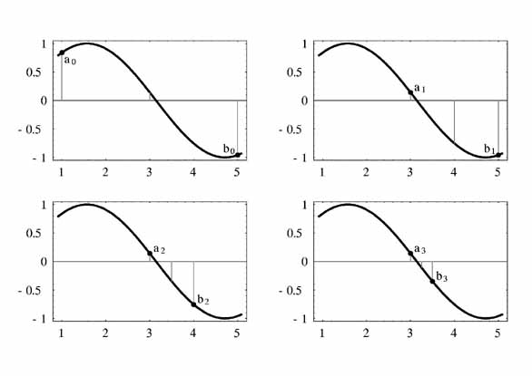
2ʬˡ��4���֤���. a_n�϶�ֻ�����n���ܤΰ���,
b_n�϶�ֽ�����n���ܤΰ���. ���ʤǤ������ΰ��֤⼨���Ƥ���.
- Solver: gsl_root_fsolver_falsepos
-
false position ���르�ꥺ���������䴰�ˤ���õ��ˡ�Ǥ���. ��«��
��������, ���̤�2ʬˡ����ᤤ.
���ʤ�, ü��(a,f(a)), (b,f(b))����ľ����������, x
���Ȥθ�����������פȤ���. �������Ǥδؿ��ͤ�������, �������Ǥɤ���
���ΰ����Ѥ��뤫����ꤷ, ������ΤƻĤ���ΰ�Ȥ���. ���Υץ�����
���㤬��֤���ʬ�˾������ʤ�ޤǷ����֤����.
���ߤο����ͤ������䴰�ˤ�������.
- Solver: gsl_root_fsolver_brent
-
Brent-Dekkerˡ(Brentˡ��ά�����Ȥˤ���)��2ʬˡ���르�ꥺ���
���ޤ��Ȥߤ��碌����ΤǤ���. ������ˡ�ϹӤäݤ����ᤤ���르�ꥺ��Ǥ���.
���ʤ�Brentˡ���������Ǵؿ���������. ���ʤǤ�2ü����ľ���������, ��
���ʤ�ˤĤ� �ǿ���3���ˤĤ��Ƶ�2��ե��åȤ�Ԥ�. ��������x��
�θ������ο����ͤȤ���. �����ͤ����ߤο����֤ˤ���������������Ѥ�,
��֤�̾�����. �������������ʤ������̾��2ʬˡ���ڤ꤫����.
�ǿ��ο����ͤϺǿ������ޤ⤷����2ʬˡ���ͤǤ���.
���ξϤ���������������ˡ�ϲ�ΰ��֤餫������ꤷ�Ƥ���ɬ�פ�����.
��«����Ȥ�������Ū���ݾڤϤʤ�--�ؿ��Ϥ��μ�ˡ��Ŭ�������Ƥ��ʤ���
�Ϥʤ餺, ����ͤϿ��β�˽�ʬ��ʤ���Фʤ�ʤ�. ��郎�������줿�Ȥ�
�ˤϼ�«��2���Ǥ���.
�����Υ��르�ꥺ��ϴؿ��Ȥ���Ƴ�ؿ���ɬ�פȤʤ�.
- Derivative Solver: gsl_root_fdfsolver_newton
-
Newtonˡ��ɸ��Ū�ʲ��������르�ꥺ��Ǥ���. ���Υ��르�ꥺ��ϲ�ΰ��֤�
��������ͤ���Ϥޤ�. ���ʤ�, �ؿ�f���������Ҥ����. ������
x���θ����������������ͤȤʤ�. �����֤��ϼ��ο������������:
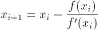
Newtonˡ��ñ��β���Ф��Ƥ�2����, ʣ���β�ˤ������Ǽ�«����.
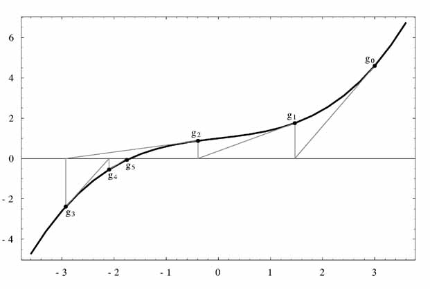
Newtonˡ�Ǥο���η����֤�. g_n��n���ܤο����ͤǤ���.
- Derivative Solver: gsl_root_fdfsolver_secant
-
����ˡ��Newtonˡ��ñ�㲽������Τ�, Ƴ�ؿ���������ɬ�פ��ʤ�.
���ʤǤϥ��르�ꥺ���Newtonˡ����Ϥ�, Ƴ�ؿ����Ѥ���.
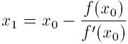
³�������֤��Ǥ�, ��ʬ�ͤ��������˿���Ū�ʿ����ͤ����Ѥ���. ����2
���η�����Ȥ����Ȥˤʤ�:
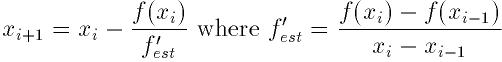
Ƴ�ؿ�����ζ�˵�Ǥ��ۤ��Ѳ����ʤ��Ȥ��ˤ�, ����ˡ�Ϥ��ʤ�ξ��ϲ���ޤ�
���Ȥ��Ǥ���. Ƴ�ؿ���ɾ�����ؿ����Ȥ�ɾ����ꥳ���Ȥ�0.44�ܰʾ夫�����
�Ǥ����, ����ˡ�ϥ˥塼�ȥ�ˡ����ᤤ. ������ʬ�η���Ʊ��, 2���δֳ�
���������ʤꤹ����ȷ������������.
ñ��β�Ǥ����, ��«��
 (��1.62)���Ǥ���. ʣ���β�Ǥ������Ǽ�«����.
- Derivative Solver: gsl_root_fdfsolver_steffenson
-
Steffensonˡ�Ϥ����롼�������ǺǤ��ᤤ��«��. ����ϴ���Ū
��Newtonˡ��Aitken�Ρ֥ǥ륿2��ײ�®���Ȥߤ��碌����ΤǤ���. Newtonˡ
�γ��ʤ�x_i�Ȥ����Ȥ�, ��®�ˤ�꿷��������R_i����������:
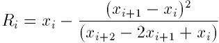
����Ϲ���Ū�ʾ��Τ�ȤǸ��ο���������«����. ��®�������������
�ˤϺ���3��ɬ�פǤ���. ���ʤǤϸ���Newtonˡ�η�̤��֤�. ��®���ʬ�줬0
�ˤʤ����Newtonˡ�η�̤��֤�.
��®�ץ�����������Ѥ��Ƥ��뤿��, �ؿ��ο����������ˤϤ�����ˡ����
����ˤʤ�.
�ɤβ�õ��ˡ�Ǥ��äƤ�, �٤����������Ѱդ���ɬ�פ�����. ������Ǥ�,
���˼��������̤�2������������Ȥˤ��褦. �ޤ��ؿ��Υѥ��������
���뤿��˥إå��ե�����(`demo_fn.h')��ɬ�פǤ���.
struct quadratic_params
  {
    double a, b, c;
  };

double quadratic (double x, void *params);
double quadratic_deriv (double x, void *params);
void quadratic_fdf (double x, void *params,
                    double *y, double *dy);
�ؿ���������̤Υե�����(`demo_fn.c')�ǹԤ����Ȥˤ��褦.
double
quadratic (double x, void *params)
{
  struct quadratic_params *p
    = (struct quadratic_params *) params;

  double a = p->a;
  double b = p->b;
  double c = p->c;

  return (a * x + b) * x + c;
}

double
quadratic_deriv (double x, void *params)
{
  struct quadratic_params *p
    = (struct quadratic_params *) params;

  double a = p->a;
  double b = p->b;
  double c = p->c;

  return 2.0 * a * x + b;
}

void
quadratic_fdf (double x, void *params,
               double *y, double *dy)
{
  struct quadratic_params *p
    = (struct quadratic_params *) params;

  double a = p->a;
  double b = p->b;
  double c = p->c;

  *y = (a * x + b) * x + c;
  *dy = 2.0 * a * x + b;
}
�ǽ�Υץ�������Brentˡ�Υ����gsl_root_fsolver_brent���Ѥ�, ��
�����������ΤǤ���.
����
 �Ǥ���.
#include <stdio.h>
#include <gsl/gsl_errno.h>
#include <gsl/gsl_math.h>
#include <gsl/gsl_roots.h>
#include "demo_fn.h"
#include "demo_fn.c"
int
main (void)
{
int status;
int iter = 0, max_iter = 100;
const gsl_root_fsolver_type *T;
gsl_root_fsolver *s;
double r = 0, r_expected = sqrt (5.0);
double x_lo = 0.0, x_hi = 5.0;
gsl_function F;
struct quadratic_params params = {1.0, 0.0, -5.0};
F.function = &quadratic;
F.params = ¶ms;
T = gsl_root_fsolver_brent;
s = gsl_root_fsolver_alloc (T);
gsl_root_fsolver_set (s, &F, x_lo, x_hi);
printf ("using %s method\n",
gsl_root_fsolver_name (s));
printf ("%5s [%9s, %9s] %9s %10s %9s\n",
"iter", "lower", "upper", "root",
"err", "err(est)");
do
{
iter++;
status = gsl_root_fsolver_iterate (s);
r = gsl_root_fsolver_root (s);
x_lo = gsl_root_fsolver_x_lower (s);
x_hi = gsl_root_fsolver_x_upper (s);
status = gsl_root_test_interval (x_lo, x_hi,
0, 0.001);
if (status == GSL_SUCCESS)
printf ("Converged:\n");
printf ("%5d [%.7f, %.7f] %.7f %+.7f %.7f\n",
iter, x_lo, x_hi,
r, r - r_expected,
x_hi - x_lo);
}
while (status == GSL_CONTINUE && iter < max_iter);
return status;
}
�ʲ��˷�̤��:
bash$ ./a.out
using brent method
 iter [    lower,     upper]      root        err  err(est)
    1 [1.0000000, 5.0000000] 1.0000000 -1.2360680 4.0000000
    2 [1.0000000, 3.0000000] 3.0000000 +0.7639320 2.0000000
    3 [2.0000000, 3.0000000] 2.0000000 -0.2360680 1.0000000
    4 [2.2000000, 3.0000000] 2.2000000 -0.0360680 0.8000000
    5 [2.2000000, 2.2366300] 2.2366300 +0.0005621 0.0366300
Converged:
    6 [2.2360634, 2.2366300] 2.2360634 -0.0000046 0.0005666
Brentˡ�ǤϤʤ�2ʬˡ��Ȥ��褦�ˤ������,
gsl_root_fsolver_brent��gsl_root_fsolver_bisection���ѹ���
��Ф褤. ���ξ��, ��«���٤��ʤ�:
bash$ ./a.out
using bisection method
 iter [    lower,     upper]      root        err  err(est)
    1 [0.0000000, 2.5000000] 1.2500000 -0.9860680 2.5000000
    2 [1.2500000, 2.5000000] 1.8750000 -0.3610680 1.2500000
    3 [1.8750000, 2.5000000] 2.1875000 -0.0485680 0.6250000
    4 [2.1875000, 2.5000000] 2.3437500 +0.1076820 0.3125000
    5 [2.1875000, 2.3437500] 2.2656250 +0.0295570 0.1562500
    6 [2.1875000, 2.2656250] 2.2265625 -0.0095055 0.0781250
    7 [2.2265625, 2.2656250] 2.2460938 +0.0100258 0.0390625
    8 [2.2265625, 2.2460938] 2.2363281 +0.0002601 0.0195312
    9 [2.2265625, 2.2363281] 2.2314453 -0.0046227 0.0097656
   10 [2.2314453, 2.2363281] 2.2338867 -0.0021813 0.0048828
   11 [2.2338867, 2.2363281] 2.2351074 -0.0009606 0.0024414
Converged:
   12 [2.2351074, 2.2363281] 2.2357178 -0.0003502 0.0012207
���Υץ�������Ʊ���ؿ���Ƴ�ؿ����Ѥ��Ʋ��õ�������ΤǤ���.
#include <stdio.h>
#include <gsl/gsl_errno.h>
#include <gsl/gsl_math.h>
#include <gsl/gsl_roots.h>
#include "demo_fn.h"
#include "demo_fn.c"
int
main (void)
{
int status;
int iter = 0, max_iter = 100;
const gsl_root_fdfsolver_type *T;
gsl_root_fdfsolver *s;
double x0, x = 5.0, r_expected = sqrt (5.0);
gsl_function_fdf FDF;
struct quadratic_params params = {1.0, 0.0, -5.0};
FDF.f = &quadratic;
FDF.df = &quadratic_deriv;
FDF.fdf = &quadratic_fdf;
FDF.params = ¶ms;
T = gsl_root_fdfsolver_newton;
s = gsl_root_fdfsolver_alloc (T);
gsl_root_fdfsolver_set (s, &FDF, x);
printf ("using %s method\n",
gsl_root_fdfsolver_name (s));
printf ("%-5s %10s %10s %10s\n",
"iter", "root", "err", "err(est)");
do
{
iter++;
status = gsl_root_fdfsolver_iterate (s);
x0 = x;
x = gsl_root_fdfsolver_root (s);
status = gsl_root_test_delta (x, x0, 0, 1e-3);
if (status == GSL_SUCCESS)
printf ("Converged:\n");
printf ("%5d %10.7f %+10.7f %10.7f\n",
iter, x, x - r_expected, x - x0);
}
while (status == GSL_CONTINUE && iter < max_iter);
return status;
}
Newtonˡ�η�̤�ʲ��˵�:
bash$ ./a.out
using newton method
iter        root        err   err(est)
    1  3.0000000 +0.7639320 -2.0000000
    2  2.3333333 +0.0972654 -0.6666667
    3  2.2380952 +0.0020273 -0.0952381
Converged:
    4  2.2360689 +0.0000009 -0.0020263
�����������ʤȤκ������꼡���ʤȤκ���Ȥ�����������ΤȤʤ�.
gsl_root_fdfsolver_newton��gsl_root_fdfsolver_secant��
gsl_root_fdfsolver_steffenson���Ѥ��뤳�Ȥ�¾����ˡ���ڤ꤫���뤳
�Ȥ��Ǥ���.
Brent-Dekker���르�ꥺ��ˤĤ��Ƥϰʲ���2�Ĥ���ʸ�Ȥ��뤳��.
-
R. P. Brent, "An algorithm with guaranteed convergence for finding a
zero of a function", Computer Journal, 14 (1971) 422-425
-
J. C. P. Bus and T. J. Dekker, "Two Efficient Algorithms with Guaranteed
Convergence for Finding a Zero of a Function", ACM Transactions of
Mathematical Software, Vol. 1 No. 4 (1975) 330-345
This chapter describes routines for finding minima of arbitrary
one-dimensional functions. The library provides low level components
for a variety of iterative minimizers and convergence tests. These can be
combined by the user to achieve the desired solution, with full access
to the intermediate steps of the algorithms. Each class of methods uses
the same framework, so that you can switch between minimizers at runtime
without needing to recompile your program. Each instance of a minimizer
keeps track of its own state, allowing the minimizers to be used in
multi-threaded programs.
The header file `gsl_min.h' contains prototypes for the
minimization functions and related declarations. To use the minimization
algorithms to find the maximum of a function simply invert its sign.
The minimization algorithms begin with a bounded region known to contain
a minimum. The region is described by an lower bound a and an
upper bound b, with an estimate of the minimum x.
![min-interval}]()
The value of the function at x must be less than the value of the
function at the ends of the interval,
This condition guarantees that a minimum is contained somewhere within
the interval. On each iteration a new point x' is selected using
one of the available algorithms. If the new point is a better estimate
of the minimum, f(x') < f(x), then the current estimate of the
minimum x is updated. The new point also allows the size of the
bounded interval to be reduced, by choosing the most compact set of
points which satisfies the constraint f(a) > f(x) < f(b). The
interval is reduced until it encloses the true minimum to a desired
tolerance. This provides a best estimate of the location of the minimum
and a rigorous error estimate.
Several bracketing algorithms are available within a single framework.
The user provides a high-level driver for the algorithm, and the
library provides the individual functions necessary for each of the
steps. There are three main phases of the iteration. The steps are,
-
initialize minimizer state, s, for algorithm T
-
update s using the iteration T
-
test s for convergence, and repeat iteration if necessary
The state for the minimizers is held in a gsl_min_fminimizer
struct. The updating procedure uses only function evaluations (not
derivatives).
Note that minimization functions can only search for one minimum at a
time. When there are several minima in the search area, the first
minimum to be found will be returned; however it is difficult to predict
which of the minima this will be. In most cases, no error will be
reported if you try to find a minimum in an area where there is more
than one.
With all minimization algorithms it can be difficult to determine the
location of the minimum to full numerical precision. The behavior of the
function in the region of the minimum x^* can be approximated by
a Taylor expansion,
and the second term of this expansion can be lost when added to the
first term at finite precision. This magnifies the error in locating
x^*, making it proportional to \sqrt \epsilon (where
\epsilon is the relative accuracy of the floating point numbers).
For functions with higher order minima, such as x^4, the
magnification of the error is correspondingly worse. The best that can
be achieved is to converge to the limit of numerical accuracy in the
function values, rather than the location of the minimum itself.
- Function: gsl_min_fminimizer * gsl_min_fminimizer_alloc (const gsl_min_fminimizer_type * T)
-
This function returns a pointer to a a newly allocated instance of a
minimizer of type T. For example, the following code
creates an instance of a golden section minimizer,
const gsl_min_fminimizer_type * T
  = gsl_min_fminimizer_goldensection;
gsl_min_fminimizer * s
  = gsl_min_fminimizer_alloc (T);
If there is insufficient memory to create the minimizer then the function
returns a null pointer and the error handler is invoked with an error
code of GSL_ENOMEM.
- Function: int gsl_min_fminimizer_set (gsl_min_fminimizer * s, gsl_function * f, double minimum, double x_lower, double x_upper)
-
This function sets, or resets, an existing minimizer s to use the
function f and the initial search interval [x_lower,
x_upper], with a guess for the location of the minimum
minimum.
If the interval given does not contain a minimum, then the function
returns an error code of GSL_FAILURE.
- Function: int gsl_min_fminimizer_set_with_values (gsl_min_fminimizer * s, gsl_function * f, double minimum, double f_minimum, double x_lower, double f_lower, double x_upper, double f_upper)
-
This function is equivalent to
gsl_min_fminimizer_set but uses
the values f_minimum, f_lower and f_upper instead of
computing f(minimum), f(x_lower) and f(x_upper).
- Function: void gsl_min_fminimizer_free (gsl_min_fminimizer * s)
-
This function frees all the memory associated with the minimizer
s.
- Function: const char * gsl_min_fminimizer_name (const gsl_min_fminimizer * s)
-
This function returns a pointer to the name of the minimizer. For example,
printf("s is a '%s' minimizer\n",
       gsl_min_fminimizer_name (s));
would print something like s is a 'brent' minimizer.
You must provide a continuous function of one variable for the
minimizers to operate on. In order to allow for general parameters the
functions are defined by a gsl_function data type
(see section Providing the function to solve).
The following functions drive the iteration of each algorithm. Each
function performs one iteration to update the state of any minimizer of the
corresponding type. The same functions work for all minimizers so that
different methods can be substituted at runtime without modifications to
the code.
- Function: int gsl_min_fminimizer_iterate (gsl_min_fminimizer * s)
-
This function performs a single iteration of the minimizer s. If the
iteration encounters an unexpected problem then an error code will be
returned,
GSL_EBADFUNC
-
the iteration encountered a singular point where the function evaluated
to
Inf or NaN.
GSL_FAILURE
-
the algorithm could not improve the current best approximation or
bounding interval.
The minimizer maintains a current best estimate of the minimum at all
times, and the current interval bounding the minimum. This information
can be accessed with the following auxiliary functions,
- Function: double gsl_min_fminimizer_minimum (const gsl_min_fminimizer * s)
-
This function returns the current estimate of the minimum for the minimizer
s.
- Function: double gsl_interval gsl_min_fminimizer_x_upper (const gsl_min_fminimizer * s)
-
- Function: double gsl_interval gsl_min_fminimizer_x_lower (const gsl_min_fminimizer * s)
-
These functions return the current upper and lower bound of the interval
for the minimizer s.
A minimization procedure should stop when one of the following
conditions is true:
-
A minimum has been found to within the user-specified precision.
-
A user-specified maximum number of iterations has been reached.
-
An error has occurred.
The handling of these conditions is under user control. The function
below allows the user to test the precision of the current result.
- Function: int gsl_min_test_interval (double x_lower, double x_upper, double epsrel, double epsabs)
-
This function tests for the convergence of the interval [x_lower,
x_upper] with absolute error epsabs and relative error
epsrel. The test returns
GSL_SUCCESS if the following
condition is achieved,
when the interval x = [a,b] does not include the origin. If the
interval includes the origin then \min(|a|,|b|) is replaced by
zero (which is the minimum value of |x| over the interval). This
ensures that the relative error is accurately estimated for minima close
to the origin.
This condition on the interval also implies that any estimate of the
minimum x_m in the interval satisfies the same condition with respect
to the true minimum x_m^*,
assuming that the true minimum x_m^* is contained within the interval.
The minimization algorithms described in this section require an initial
interval which is guaranteed to contain a minimum -- if a and
b are the endpoints of the interval and x is an estimate
of the minimum then f(a) > f(x) < f(b). This ensures that the
function has at least one minimum somewhere in the interval. If a valid
initial interval is used then these algorithm cannot fail, provided the
function is well-behaved.
- Minimizer: gsl_min_fminimizer_goldensection
-
The golden section algorithm is the simplest method of bracketing
the minimum of a function. It is the slowest algorithm provided by the
library, with linear convergence.
On each iteration, the algorithm first compares the subintervals from
the endpoints to the current minimum. The larger subinterval is divided
in a golden section (using the famous ratio (3-\sqrt 5)/2 =
0.3189660...) and the value of the function at this new point is
calculated. The new value is used with the constraint f(a') >
f(x') < f(b') to a select new interval containing the minimum, by
discarding the least useful point. This procedure can be continued
indefinitely until the interval is sufficiently small. Choosing the
golden section as the bisection ratio can be shown to provide the
fastest convergence for this type of algorithm.
- Minimizer: gsl_min_fminimizer_brent
-
The Brent minimization algorithm combines a parabolic
interpolation with the golden section algorithm. This produces a fast
algorithm which is still robust.
The outline of the algorithm can be summarized as follows: on each
iteration Brent's method approximates the function using an
interpolating parabola through three existing points. The minimum of the
parabola is taken as a guess for the minimum. If it lies within the
bounds of the current interval then the interpolating point is accepted,
and used to generate a smaller interval. If the interpolating point is
not accepted then the algorithm falls back to an ordinary golden section
step. The full details of Brent's method include some additional checks
to improve convergence.
The following program uses the Brent algorithm to find the minimum of
the function f(x) = \cos(x) + 1, which occurs at x = \pi.
The starting interval is (0,6), with an initial guess for the
minimum of 2.
#include <stdio.h>
#include <gsl/gsl_errno.h>
#include <gsl/gsl_math.h>
#include <gsl/gsl_min.h>

double fn1 (double x, void * params)
{
  return cos(x) + 1.0;
}

int
main (void)
{
  int status;
  int iter = 0, max_iter = 100;
  const gsl_min_fminimizer_type *T;
  gsl_min_fminimizer *s;
  double m = 2.0, m_expected = M_PI;
  double a = 0.0, b = 6.0;
  gsl_function F;

  F.function = &fn1;
  F.params = 0;

  T = gsl_min_fminimizer_brent;
  s = gsl_min_fminimizer_alloc (T);
  gsl_min_fminimizer_set (s, &F, m, a, b);

  printf ("using %s method\n",
          gsl_min_fminimizer_name (s));

  printf ("%5s [%9s, %9s] %9s %10s %9s\n",
          "iter", "lower", "upper", "min",
          "err", "err(est)");

  printf ("%5d [%.7f, %.7f] %.7f %+.7f %.7f\n",
          iter, a, b,
          m, m - m_expected, b - a);

  do
    {
      iter++;
      status = gsl_min_fminimizer_iterate (s);

      m = gsl_min_fminimizer_minimum (s);
      a = gsl_min_fminimizer_x_lower (s);
      b = gsl_min_fminimizer_x_upper (s);

      status
        = gsl_min_test_interval (a, b, 0.001, 0.0);

      if (status == GSL_SUCCESS)
        printf ("Converged:\n");

      printf ("%5d [%.7f, %.7f] "
              "%.7f %.7f %+.7f %.7f\n",
              iter, a, b,
              m, m_expected, m - m_expected, b - a);
    }
  while (status == GSL_CONTINUE && iter < max_iter);

  return status;
}
Here are the results of the minimization procedure.
bash$ ./a.out
    0 [0.0000000, 6.0000000] 2.0000000 -1.1415927 6.0000000
    1 [2.0000000, 6.0000000] 3.2758640 +0.1342713 4.0000000
    2 [2.0000000, 3.2831929] 3.2758640 +0.1342713 1.2831929
    3 [2.8689068, 3.2831929] 3.2758640 +0.1342713 0.4142862
    4 [2.8689068, 3.2831929] 3.2758640 +0.1342713 0.4142862
    5 [2.8689068, 3.2758640] 3.1460585 +0.0044658 0.4069572
    6 [3.1346075, 3.2758640] 3.1460585 +0.0044658 0.1412565
    7 [3.1346075, 3.1874620] 3.1460585 +0.0044658 0.0528545
    8 [3.1346075, 3.1460585] 3.1460585 +0.0044658 0.0114510
    9 [3.1346075, 3.1460585] 3.1424060 +0.0008133 0.0114510
   10 [3.1346075, 3.1424060] 3.1415885 -0.0000041 0.0077985
Converged:
   11 [3.1415885, 3.1424060] 3.1415927 -0.0000000 0.0008175
Further information on Brent's algorithm is available in the following
book,
-
Richard Brent, Algorithms for minimization without derivatives,
Prentice-Hall (1973)
This chapter describes functions for multidimensional root-finding
(solving nonlinear systems with n equations in n
unknowns). The library provides low level components for a variety of
iterative solvers and convergence tests. These can be combined by the
user to achieve the desired solution, with full access to the
intermediate steps of the iteration. Each class of methods uses the
same framework, so that you can switch between solvers at runtime
without needing to recompile your program. Each instance of a solver
keeps track of its own state, allowing the solvers to be used in
multi-threaded programs. The solvers are based on the original Fortran
library MINPACK.
The header file `gsl_multiroots.h' contains prototypes for the
multidimensional root finding functions and related declarations.
The problem of multidimensional root finding requires the simultaneous
solution of n equations, f_i, in n variables,
x_i,
In general there are no bracketing methods available for n
dimensional systems, and no way of knowing whether any solutions
exist. All algorithms proceed from an initial guess using a variant of
the Newton iteration,
where x, f are vector quantities and J is the
Jacobian matrix @c{$J_{ij} = \partial f_i / \partial x_j$}
J_{ij} = d f_i / d x_j.
Additional strategies can be used to enlarge the region of
convergence. These include requiring a decrease in the norm |f| on
each step proposed by Newton's method, or taking steepest-descent steps in
the direction of the negative gradient of |f|.
Several root-finding algorithms are available within a single framework.
The user provides a high-level driver for the algorithms, and the
library provides the individual functions necessary for each of the
steps. There are three main phases of the iteration. The steps are,
-
initialize solver state, s, for algorithm T
-
update s using the iteration T
-
test s for convergence, and repeat iteration if necessary
The evaluation of the Jacobian matrix can be problematic, either because
programming the derivatives is intractable or because computation of the
n^2 terms of the matrix becomes too expensive. For these reasons
the algorithms provided by the library are divided into two classes according
to whether the derivatives are available or not.
The state for solvers with an analytic Jacobian matrix is held in a
gsl_multiroot_fdfsolver struct. The updating procedure requires
both the function and its derivatives to be supplied by the user.
The state for solvers which do not use an analytic Jacobian matrix is
held in a gsl_multiroot_fsolver struct. The updating procedure
uses only function evaluations (not derivatives). The algorithms
estimate the matrix J or @c{$J^{-1}$}
J^{-1} by approximate methods.
The following functions initialize a multidimensional solver, either
with or without derivatives. The solver itself depends only on the
dimension of the problem and the algorithm and can be reused for
different problems.
- Function: gsl_multiroot_fsolver * gsl_multiroot_fsolver_alloc (const gsl_multiroot_fsolver_type * T, size_t n)
-
This function returns a pointer to a a newly allocated instance of a
solver of type T for a system of n dimensions.
For example, the following code creates an instance of a hybrid solver,
to solve a 3-dimensional system of equations.
const gsl_multiroot_fsolver_type * T
    = gsl_multiroot_fsolver_hybrid;
gsl_multiroot_fsolver * s
    = gsl_multiroot_fsolver_alloc (T, 3);
If there is insufficient memory to create the solver then the function
returns a null pointer and the error handler is invoked with an error
code of GSL_ENOMEM.
- Function: gsl_multiroot_fdfsolver * gsl_multiroot_fdfsolver_alloc (const gsl_multiroot_fdfsolver_type * T, size_t n)
-
This function returns a pointer to a a newly allocated instance of a
derivative solver of type T for a system of n dimensions.
For example, the following code creates an instance of a Newton-Raphson solver,
for a 2-dimensional system of equations.
const gsl_multiroot_fdfsolver_type * T
    = gsl_multiroot_fdfsolver_newton;
gsl_multiroot_fdfsolver * s =
    gsl_multiroot_fdfsolver_alloc (T, 2);
If there is insufficient memory to create the solver then the function
returns a null pointer and the error handler is invoked with an error
code of GSL_ENOMEM.
- Function: int gsl_multiroot_fsolver_set (gsl_multiroot_fsolver * s, gsl_multiroot_function * f, gsl_vector * x)
-
This function sets, or resets, an existing solver s to use the
function f and the initial guess x.
- Function: int gsl_multiroot_fdfsolver_set (gsl_multiroot_fdfsolver * s, gsl_function_fdf * fdf, gsl_vector * x)
-
This function sets, or resets, an existing solver s to use the
function and derivative fdf and the initial guess x.
- Function: void gsl_multiroot_fsolver_free (gsl_multiroot_fsolver * s)
-
- Function: void gsl_multiroot_fdfsolver_free (gsl_multiroot_fdfsolver * s)
-
These functions free all the memory associated with the solver s.
- Function: const char * gsl_multiroot_fsolver_name (const gsl_multiroot_fsolver * s)
-
- Function: const char * gsl_multiroot_fdfsolver_name (const gsl_multiroot_fdfsolver * s)
-
These functions return a pointer to the name of the solver. For example,
printf("s is a '%s' solver\n",
       gsl_multiroot_fdfsolver_name (s));
would print something like s is a 'newton' solver.
You must provide n functions of n variables for the root
finders to operate on. In order to allow for general parameters the
functions are defined by the following data types:
- Data Type: gsl_multiroot_function
-
This data type defines a general system of functions with parameters.
int (* f) (const gsl_vector * x, void * params, gsl_vector * f)
-
this function should store the vector result
f(x,params) in f for argument x and parameters params,
returning an appropriate error code if the function cannot be computed.
size_t n
-
the dimension of the system, i.e. the number of components of the
vectors x and f.
void * params
-
a pointer to the parameters of the function.
Here is an example using Powell's test function,
with A = 10^4. The following code defines a
gsl_multiroot_function system F which you could pass to a
solver:
struct powell_params { double A; };
int
powell (gsl_vector * x, void * p, gsl_vector * f) {
struct powell_params * params
= *(struct powell_params *)p;
double A = (params->A);
double x0 = gsl_vector_get(x,0);
double x1 = gsl_vector_get(x,1);
gsl_vector_set (f, 0, A * x0 * x1 - 1)
gsl_vector_set (f, 1, (exp(-x0) + exp(-x1)
- (1.0 + 1.0/A)))
return GSL_SUCCESS
}
gsl_multiroot_function F;
struct powell_params params = { 10000.0 };
F.function = &powell;
F.n = 2;
F.params = ¶ms;
- Data Type: gsl_multiroot_function_fdf
-
This data type defines a general system of functions with parameters and
the corresponding Jacobian matrix of derivatives,
int (* f) (const gsl_vector * x, void * params, gsl_vector * f)
-
this function should store the vector result
f(x,params) in f for argument x and parameters params,
returning an appropriate error code if the function cannot be computed.
int (* df) (const gsl_vector * x, void * params, gsl_matrix * J)
-
this function should store the n-by-n matrix result
J_ij = d f_i(x,params) / d x_j in J for argument x
and parameters params, returning an appropriate error code if the
function cannot be computed.
int (* fdf) (const gsl_vector * x, void * params, gsl_vector * f, gsl_matrix * J)
-
This function should set the values of the f and J as above,
for arguments x and parameters params. This function provides
an optimization of the separate functions for f(x) and J(x) --
it is always faster to compute the function and its derivative at the
same time.
size_t n
-
the dimension of the system, i.e. the number of components of the
vectors x and f.
void * params
-
a pointer to the parameters of the function.
The example of Powell's test function defined above can be extended to
include analytic derivatives using the following code,
int
powell_df (gsl_vector * x, void * p, gsl_matrix * J)
{
   struct powell_params * params
     = *(struct powell_params *)p;
   double A = (params->A);
   double x0 = gsl_vector_get(x,0);
   double x1 = gsl_vector_get(x,1);
   gsl_vector_set (J, 0, 0, A * x1)
   gsl_vector_set (J, 0, 1, A * x0)
   gsl_vector_set (J, 1, 0, -exp(-x0))
   gsl_vector_set (J, 1, 1, -exp(-x1))
   return GSL_SUCCESS
}

int
powell_fdf (gsl_vector * x, void * p,
            gsl_matrix * f, gsl_matrix * J) {
   struct powell_params * params
     = *(struct powell_params *)p;
   double A = (params->A);
   double x0 = gsl_vector_get(x,0);
   double x1 = gsl_vector_get(x,1);

   double u0 = exp(-x0);
   double u1 = exp(-x1);

   gsl_vector_set (f, 0, A * x0 * x1 - 1)
   gsl_vector_set (f, 1, u0 + u1 - (1 + 1/A))

   gsl_vector_set (J, 0, 0, A * x1)
   gsl_vector_set (J, 0, 1, A * x0)
   gsl_vector_set (J, 1, 0, -u0)
   gsl_vector_set (J, 1, 1, -u1)
   return GSL_SUCCESS
}

gsl_multiroot_function_fdf FDF;

FDF.f = &powell_f;
FDF.df = &powell_df;
FDF.fdf = &powell_fdf;
FDF.n = 2;
FDF.params = 0;
Note that the function powell_fdf is able to reuse existing terms
from the function when calculating the Jacobian, thus saving time.
The following functions drive the iteration of each algorithm. Each
function performs one iteration to update the state of any solver of the
corresponding type. The same functions work for all solvers so that
different methods can be substituted at runtime without modifications to
the code.
- Function: int gsl_multiroot_fsolver_iterate (gsl_multiroot_fsolver * s)
-
- Function: int gsl_multiroot_fdfsolver_iterate (gsl_multiroot_fdfsolver * s)
-
These functions perform a single iteration of the solver s. If the
iteration encounters an unexpected problem then an error code will be
returned,
GSL_EBADFUNC
-
the iteration encountered a singular point where the function or its
derivative evaluated to
Inf or NaN.
GSL_ENOPROG
-
the iteration is not making any progress, preventing the algorithm from
continuing.
The solver maintains a current best estimate of the root at all times.
This information can be accessed with the following auxiliary functions,
- Function: gsl_vector * gsl_multiroot_fsolver_root (const gsl_multiroot_fsolver * s)
-
- Function: gsl_vector * gsl_multiroot_fdfsolver_root (const gsl_multiroot_fdfsolver * s)
-
These functions return the current estimate of the root for the solver s.
A root finding procedure should stop when one of the following conditions is
true:
-
A multidimensional root has been found to within the user-specified precision.
-
A user-specified maximum number of iterations has been reached.
-
An error has occurred.
The handling of these conditions is under user control. The functions
below allow the user to test the precision of the current result in
several standard ways.
- Function: int gsl_multiroot_test_delta (const gsl_vector * dx, const gsl_vector * x, double epsabs, double epsrel)
-
This function tests for the convergence of the sequence by comparing the
last step dx with the absolute error epsabs and relative
error epsrel to the current position x. The test returns
GSL_SUCCESS if the following condition is achieved,
for each component of x and returns GSL_CONTINUE otherwise.
- Function: int gsl_multiroot_test_residual (const gsl_vector * f, double epsabs)
-
This function tests the residual value f against the absolute
error bound epsabs. The test returns
GSL_SUCCESS if the
following condition is achieved,
and returns GSL_CONTINUE otherwise. This criterion is suitable
for situations where the the precise location of the root, x, is
unimportant provided a value can be found where the residual is small
enough.
The root finding algorithms described in this section make use of both
the function and its derivative. They require an initial guess for the
location of the root, but there is no absolute guarantee of convergence
-- the function must be suitable for this technique and the initial
guess must be sufficiently close to the root for it to work. When the
conditions are satisfied then convergence is quadratic.
- Derivative Solver: gsl_multiroot_fdfsolver_hybridsj
-
This is a modified version of Powell's Hybrid method as implemented in
the HYBRJ algorithm in MINPACK. Minpack was written by Jorge
J. Mor'e, Burton S. Garbow and Kenneth E. Hillstrom. The Hybrid
algorithm retains the fast convergence of Newton's method but will also
reduce the residual when Newton's method is unreliable.
The algorithm uses a generalized trust region to keep each step under
control. In order to be accepted a proposed new position x' must
satisfy the condition |D (x' - x)| < \delta, where D is a
diagonal scaling matrix and \delta is the size of the trust
region. The components of D are computed internally, using the
column norms of the Jacobian to estimate the sensitivity of the residual
to each component of x. This improves the behavior of the
algorithm for badly scaled functions.
On each iteration the algorithm first determines the standard Newton
step by solving the system J dx = - f. If this step falls inside
the trust region it is used as a trial step in the next stage. If not,
the algorithm uses the linear combination of the Newton and gradient
directions which is predicted to minimize the norm of the function while
staying inside the trust region.
This combination of Newton and gradient directions is referred to as a
dogleg step.
The proposed step is now tested by evaluating the function at the
resulting point, x'. If the step reduces the norm of the function
sufficiently then it is accepted and size of the trust region is
increased. If the proposed step fails to improve the solution then the
size of the trust region is decreased and another trial step is
computed.
The speed of the algorithm is increased by computing the changes to the
Jacobian approximately, using a rank-1 update. If two successive
attempts fail to reduce the residual then the full Jacobian is
recomputed. The algorithm also monitors the progress of the solution
and returns an error if several steps fail to make any improvement,
GSL_ENOPROG
-
the iteration is not making any progress, preventing the algorithm from
continuing.
GSL_ENOPROGJ
-
re-evaluations of the Jacobian indicate that the iteration is not
making any progress, preventing the algorithm from continuing.
- Derivative Solver: gsl_multiroot_fdfsolver_hybridj
-
This algorithm is an unscaled version of
hybridsj. The steps are
controlled by a spherical trust region |x' - x| < \delta, instead
of a generalized region. This can be useful if the generalized region
estimated by hybridsj is inappropriate.
- Derivative Solver: gsl_multiroot_fdfsolver_newton
-
Newton's Method is the standard root-polishing algorithm. The algorithm
begins with an initial guess for the location of the solution. On each
iteration a linear approximation to the function F is used to
estimate the step which will zero all the components of the residual.
The iteration is defined by the following sequence,
where the Jacobian matrix J is computed from the derivative
functions provided by f. The step dx is obtained by solving
the linear system,
using LU decomposition.
- Derivative Solver: gsl_multiroot_fdfsolver_gnewton
-
This is a modified version of Newton's method which attempts to improve
global convergence by requiring every step to reduce the Euclidean norm
of the residual, |f(x)|. If the Newton step leads to an increase
in the norm then a reduced step of relative size,
is proposed, with r being the ratio of norms
|f(x')|^2/|f(x)|^2. This procedure is repeated until a suitable step
size is found.
The algorithms described in this section do not require any derivative
information to be supplied by the user. Any derivatives needed are
approximated from by finite difference.
- Solver: gsl_multiroot_fsolver_hybrids
-
This is a version of the Hybrid algorithm which replaces calls to the
Jacobian function by its finite difference approximation. The finite
difference approximation is computed using
gsl_multiroots_fdjac
with a relative step size of GSL_SQRT_DBL_EPSILON.
- Solver: gsl_multiroot_fsolver_hybrid
-
This is a finite difference version of the Hybrid algorithm without
internal scaling.
- Solver: gsl_multiroot_fsolver_dnewton
-
The discrete Newton algorithm is the simplest method of solving a
multidimensional system. It uses the Newton iteration
where the Jacobian matrix J is approximated by taking finite
differences of the function f. The approximation scheme used by
this implementation is,
where \delta_j is a step of size \sqrt\epsilon |x_j| with
\epsilon being the machine precision
(@c{$\epsilon \approx 2.22 \times 10^{-16}$}
\epsilon \approx 2.22 \times 10^-16).
The order of convergence of Newton's algorithm is quadratic, but the
finite differences require n^2 function evaluations on each
iteration. The algorithm may become unstable if the finite differences
are not a good approximation to the true derivatives.
- Solver: gsl_multiroot_fsolver_broyden
-
The Broyden algorithm is a version of the discrete Newton
algorithm which attempts to avoids the expensive update of the Jacobian
matrix on each iteration. The changes to the Jacobian are also
approximated, using a rank-1 update,
where the vectors dx and df are the changes in x
and f. On the first iteration the inverse Jacobian is estimated
using finite differences, as in the discrete Newton algorithm.
This approximation gives a fast update but is unreliable if the changes
are not small, and the estimate of the inverse Jacobian becomes worse as
time passes. The algorithm has a tendency to become unstable unless it
starts close to the root. The Jacobian is refreshed if this instability
is detected (consult the source for details).
This algorithm is not recommended and is included only for demonstration
purposes.
The multidimensional solvers are used in a similar way to the
one-dimensional root finding algorithms. This first example
demonstrates the hybrids scaled-hybrid algorithm, which does not
require derivatives. The program solves the Rosenbrock system of equations,
with a = 1, b = 10. The solution of this system lies at
(x,y) = (1,1) in a narrow valley.
The first stage of the program is to define the system of equations,
#include <stdlib.h>
#include <stdio.h>
#include <gsl/gsl_vector.h>
#include <gsl/gsl_multiroots.h>

struct rparams
  {
    double a;
    double b;
  };

int
rosenbrock_f (const gsl_vector * x, void *params,
              gsl_vector * f)
{
  double a = ((struct rparams *) params)->a;
  double b = ((struct rparams *) params)->b;

  double x0 = gsl_vector_get (x, 0);
  double x1 = gsl_vector_get (x, 1);

  double y0 = a * (1 - x0);
  double y1 = b * (x1 - x0 * x0);

  gsl_vector_set (f, 0, y0);
  gsl_vector_set (f, 1, y1);

  return GSL_SUCCESS;
}
The main program begins by creating the function object f, with
the arguments (x,y) and parameters (a,b). The solver
s is initialized to use this function, with the hybrids
method.
int
main (void)
{
  const gsl_multiroot_fsolver_type *T;
  gsl_multiroot_fsolver *s;

  int status;
  size_t i, iter = 0;

  const size_t n = 2;
  struct rparams p = {1.0, 10.0};
  gsl_multiroot_function f = {&rosenbrock_f, n, &p};

  double x_init[2] = {-10.0, -5.0};
  gsl_vector *x = gsl_vector_alloc (n);

  gsl_vector_set (x, 0, x_init[0]);
  gsl_vector_set (x, 1, x_init[1]);

  T = gsl_multiroot_fsolver_hybrids;
  s = gsl_multiroot_fsolver_alloc (T, 2);
  gsl_multiroot_fsolver_set (s, &f, x);

  print_state (iter, s);

  do
    {
      iter++;
      status = gsl_multiroot_fsolver_iterate (s);

      print_state (iter, s);

      if (status)   /* check if solver is stuck */
        break;

      status =
        gsl_multiroot_test_residual (s->f, 1e-7);
    }
  while (status == GSL_CONTINUE && iter < 1000);

  printf ("status = %s\n", gsl_strerror (status));

  gsl_multiroot_fsolver_free (s);
  gsl_vector_free (x);
  return 0;
}
Note that it is important to check the return status of each solver
step, in case the algorithm becomes stuck. If an error condition is
detected, indicating that the algorithm cannot proceed, then the error
can be reported to the user, a new starting point chosen or a different
algorithm used.
The intermediate state of the solution is displayed by the following
function. The solver state contains the vector s->x which is the
current position, and the vector s->f with corresponding function
values.
int
print_state (size_t iter, gsl_multiroot_fsolver * s)
{
  printf ("iter = %3u x = % .3f % .3f "
          "f(x) = % .3e % .3e\n",
          iter,
          gsl_vector_get (s->x, 0),
          gsl_vector_get (s->x, 1),
          gsl_vector_get (s->f, 0),
          gsl_vector_get (s->f, 1));
}
Here are the results of running the program. The algorithm is started at
(-10,-5) far from the solution. Since the solution is hidden in
a narrow valley the earliest steps follow the gradient of the function
downhill, in an attempt to reduce the large value of the residual. Once
the root has been approximately located, on iteration 8, the Newton
behavior takes over and convergence is very rapid.
iter =  0 x = -10.000  -5.000  f(x) = 1.100e+01 -1.050e+03
iter =  1 x = -10.000  -5.000  f(x) = 1.100e+01 -1.050e+03
iter =  2 x =  -3.976  24.827  f(x) = 4.976e+00  9.020e+01
iter =  3 x =  -3.976  24.827  f(x) = 4.976e+00  9.020e+01
iter =  4 x =  -3.976  24.827  f(x) = 4.976e+00  9.020e+01
iter =  5 x =  -1.274  -5.680  f(x) = 2.274e+00 -7.302e+01
iter =  6 x =  -1.274  -5.680  f(x) = 2.274e+00 -7.302e+01
iter =  7 x =   0.249   0.298  f(x) = 7.511e-01  2.359e+00
iter =  8 x =   0.249   0.298  f(x) = 7.511e-01  2.359e+00
iter =  9 x =   1.000   0.878  f(x) = 1.268e-10 -1.218e+00
iter = 10 x =   1.000   0.989  f(x) = 1.124e-11 -1.080e-01
iter = 11 x =   1.000   1.000  f(x) = 0.000e+00  0.000e+00
status = success
Note that the algorithm does not update the location on every
iteration. Some iterations are used to adjust the trust-region
parameter, after trying a step which was found to be divergent, or to
recompute the Jacobian, when poor convergence behavior is detected.
The next example program adds derivative information, in order to
accelerate the solution. There are two derivative functions
rosenbrock_df and rosenbrock_fdf. The latter computes both
the function and its derivative simultaneously. This allows the
optimization of any common terms. For simplicity we substitute calls to
the separate f and df functions at this point in the code
below.
int
rosenbrock_df (const gsl_vector * x, void *params,
               gsl_matrix * J)
{
  double a = ((struct rparams *) params)->a;
  double b = ((struct rparams *) params)->b;

  double x0 = gsl_vector_get (x, 0);

  double df00 = -a;
  double df01 = 0;
  double df10 = -2 * b  * x0;
  double df11 = b;

  gsl_matrix_set (J, 0, 0, df00);
  gsl_matrix_set (J, 0, 1, df01);
  gsl_matrix_set (J, 1, 0, df10);
  gsl_matrix_set (J, 1, 1, df11);

  return GSL_SUCCESS;
}

int
rosenbrock_fdf (const gsl_vector * x, void *params,
                gsl_vector * f, gsl_matrix * J)
{
  rosenbrock_f (x, params, f);
  rosenbrock_df (x, params, J);

  return GSL_SUCCESS;
}
The main program now makes calls to the corresponding fdfsolver
versions of the functions,
int
main (void)
{
  const gsl_multiroot_fdfsolver_type *T;
  gsl_multiroot_fdfsolver *s;

  int status;
  size_t i, iter = 0;

  const size_t n = 2;
  struct rparams p = {1.0, 10.0};
  gsl_multiroot_function_fdf f = {&rosenbrock_f,
                                  &rosenbrock_df,
                                  &rosenbrock_fdf,
                                  n, &p};

  double x_init[2] = {-10.0, -5.0};
  gsl_vector *x = gsl_vector_alloc (n);

  gsl_vector_set (x, 0, x_init[0]);
  gsl_vector_set (x, 1, x_init[1]);

  T = gsl_multiroot_fdfsolver_gnewton;
  s = gsl_multiroot_fdfsolver_alloc (T, n);
  gsl_multiroot_fdfsolver_set (s, &f, x);

  print_state (iter, s);

  do
    {
      iter++;

      status = gsl_multiroot_fdfsolver_iterate (s);

      print_state (iter, s);

      if (status)
        break;

      status = gsl_multiroot_test_residual (s->f, 1e-7);
    }
  while (status == GSL_CONTINUE && iter < 1000);

  printf ("status = %s\n", gsl_strerror (status));

  gsl_multiroot_fdfsolver_free (s);
  gsl_vector_free (x);
  return 0;
}
The addition of derivative information to the hybrids solver does
not make any significant difference to its behavior, since it able to
approximate the Jacobian numerically with sufficient accuracy. To
illustrate the behavior of a different derivative solver we switch to
gnewton. This is a traditional newton solver with the constraint
that it scales back its step if the full step would lead "uphill". Here
is the output for the gnewton algorithm,
iter = 0 x = -10.000  -5.000 f(x) =  1.100e+01 -1.050e+03
iter = 1 x =  -4.231 -65.317 f(x) =  5.231e+00 -8.321e+02
iter = 2 x =   1.000 -26.358 f(x) = -8.882e-16 -2.736e+02
iter = 3 x =   1.000   1.000 f(x) = -2.220e-16 -4.441e-15
status = success
The convergence is much more rapid, but takes a wide excursion out to
the point (-4.23,-65.3). This could cause the algorithm to go
astray in a realistic application. The hybrid algorithm follows the
downhill path to the solution more reliably.
The original version of the Hybrid method is described in the following
articles by Powell,
-
M.J.D. Powell, "A Hybrid Method for Nonlinear Equations" (Chap 6, p
87-114) and "A Fortran Subroutine for Solving systems of Nonlinear
Algebraic Equations" (Chap 7, p 115-161), in Numerical Methods for
Nonlinear Algebraic Equations, P. Rabinowitz, editor. Gordon and
Breach, 1970.
The following papers are also relevant to the algorithms described in
this section,
-
J.J. Mor'e, M.Y. Cosnard, "Numerical Solution of Nonlinear Equations",
ACM Transactions on Mathematical Software, Vol 5, No 1, (1979), p 64-85
-
C.G. Broyden, "A Class of Methods for Solving Nonlinear
Simultaneous Equations", Mathematics of Computation, Vol 19 (1965),
p 577-593
-
J.J. Mor'e, B.S. Garbow, K.E. Hillstrom, "Testing Unconstrained
Optimization Software", ACM Transactions on Mathematical Software, Vol
7, No 1 (1981), p 17-41
This chapter describes routines for finding minima of arbitrary
multidimensional functions. The library provides low level components
for a variety of iterative minimizers and convergence tests. These can
be combined by the user to achieve the desired solution, while providing
full access to the intermediate steps of the algorithms. Each class of
methods uses the same framework, so that you can switch between
minimizers at runtime without needing to recompile your program. Each
instance of a minimizer keeps track of its own state, allowing the
minimizers to be used in multi-threaded programs. The minimization
algorithms can be used to maximize a function by inverting its sign.
The header file `gsl_multimin.h' contains prototypes for the
minimization functions and related declarations.
The problem of multidimensional minimization requires finding a point
x such that the scalar function,
takes a value which is lower than at any neighboring point. For smooth
functions the gradient g = \nabla f vanishes at the minimum. In
general there are no bracketing methods available for the minimization
of n-dimensional functions. All algorithms proceed from an
initial guess using a search algorithm which attempts to move in a
downhill direction. A one-dimensional line minimisation is performed
along this direction until the lowest point is found to a suitable
tolerance. The search direction is then updated with local information
from the function and its derivatives, and the whole process repeated
until the true n-dimensional minimum is found.
Several minimization algorithms are available within a single
framework. The user provides a high-level driver for the algorithms, and
the library provides the individual functions necessary for each of the
steps. There are three main phases of the iteration. The steps are,
-
initialize minimizer state, s, for algorithm T
-
update s using the iteration T
-
test s for convergence, and repeat iteration if necessary
Each iteration step consists either of an improvement to the
line-mimisation in the current direction or an update to the search
direction itself. The state for the minimizers is held in a
gsl_multimin_fdfminimizer struct.
Note that the minimization algorithms can only search for one local
minimum at a time. When there are several local minima in the search
area, the first minimum to be found will be returned; however it is
difficult to predict which of the minima this will be. In most cases,
no error will be reported if you try to find a local minimum in an area
where there is more than one.
It is also important to note that the minimization algorithms find local
minima; there is no way to determine whether a minimum is a global
minimum of the function in question.
The following function initializes a multidimensional minimizer. The
minimizer itself depends only on the dimension of the problem and the
algorithm and can be reused for different problems.
- Function: gsl_multimin_fdfminimizer * gsl_multimin_fdfminimizer_alloc (const gsl_multimin_fdfminimizer_type *T, size_t n)
-
This function returns a pointer to a a newly allocated instance of a
minimizer of type T for an n-dimension function. If there
is insufficient memory to create the minimizer then the function returns
a null pointer and the error handler is invoked with an error code of
GSL_ENOMEM.
- Function: int gsl_multimin_fdfminimizer_set (gsl_multimin_fdfminimizer * s, gsl_multimin_function_fdf *fdf, const gsl_vector * x, double step_size, double tol)
-
This function initializes the minimizer s to minimize the function
fdf starting from the initial point x. The size of the
first trial step is given by step_size. The accuracy of the line
minimization is specified by tol. The precise meaning of this
parameter depends on the method used. Typically the line minimization
is considered successful if the gradient of the function g is
orthogonal to the current search direction p to a relative
accuracy of tol, where @c{$p\cdot g < tol |p| |g|$}
dot(p,g) < tol |p| |g|.
- Function: void gsl_multimin_fdfminimizer_free (gsl_multimin_fdfminimizer *s)
-
This function frees all the memory associated with the minimizer
s.
- Function: const char * gsl_multimin_fdfminimizer_name (const gsl_multimin_fdfminimizer * s)
-
This function returns a pointer to the name of the minimizer. For example,
printf("s is a '%s' minimizer\n",
       gsl_multimin_fdfminimizer_name (s));
would print something like s is a 'conjugate_pr' minimizer.
You must provide a parametric function of n variables for the
minimizers to operate on. You also need to provide a routine which
calculates the gradient of the function and a third routine which
calculates both the function value and the gradient together. In order
to allow for general parameters the functions are defined by the
following data type:
- Data Type: gsl_multimin_function_fdf
-
This data type defines a general function of n variables with
parameters and the corresponding gradient vector of derivatives,
double (* f) (const gsl_vector * x, void * params)
-
this function should return the result
f(x,params) for argument x and parameters params.
int (* df) (const gsl_vector * x, void * params, gsl_vector * g)
-
this function should store the n-dimensional gradient
g_i = d f(x,params) / d x_i in the vector g for argument x
and parameters params, returning an appropriate error code if the
function cannot be computed.
int (* fdf) (const gsl_vector * x, void * params, double * f, gsl_vector * g)
-
This function should set the values of the f and g as above,
for arguments x and parameters params. This function provides
an optimization of the separate functions for f(x) and g(x) --
it is always faster to compute the function and its derivative at the
same time.
size_t n
-
the dimension of the system, i.e. the number of components of the
vectors x.
void * params
-
a pointer to the parameters of the function.
The following example function defines a simple paraboloid with two
parameters,
/* Paraboloid centered on (dp[0],dp[1]) */

double
my_f (const gsl_vector *v, void *params)
{
  double x, y;
  double *dp = (double *)params;

  x = gsl_vector_get(v, 0);
  y = gsl_vector_get(v, 1);

  return 10.0 * (x - dp[0]) * (x - dp[0]) +
           20.0 * (y - dp[1]) * (y - dp[1]) + 30.0;
}

/* The gradient of f, df = (df/dx, df/dy). */
void
my_df (const gsl_vector *v, void *params,
       gsl_vector *df)
{
  double x, y;
  double *dp = (double *)params;

  x = gsl_vector_get(v, 0);
  y = gsl_vector_get(v, 1);

  gsl_vector_set(df, 0, 20.0 * (x - dp[0]));
  gsl_vector_set(df, 1, 40.0 * (y - dp[1]));
}

/* Compute both f and df together. */
void
my_fdf (const gsl_vector *x, void *params,
        double *f, gsl_vector *df)
{
  *f = my_f(x, params);
  my_df(x, params, df);
}
The function can be initialized using the following code,
gsl_multimin_function_fdf my_func;

double p[2] = { 1.0, 2.0 }; /* center at (1,2) */

my_func.f = &my_f;
my_func.df = &my_df;
my_func.fdf = &my_fdf;
my_func.n = 2;
my_func.params = (void *)p;
The following function drives the iteration of each algorithm. The
function performs one iteration to update the state of the minimizer.
The same function works for all minimizers so that different methods can
be substituted at runtime without modifications to the code.
- Function: int gsl_multimin_fdfminimizer_iterate (gsl_multimin_fdfminimizer *s)
-
These functions perform a single iteration of the minimizer s. If
the iteration encounters an unexpected problem then an error code will
be returned.
The minimizer maintains a current best estimate of the minimum at all
times. This information can be accessed with the following auxiliary
functions,
- Function: gsl_vector * gsl_multiroot_fdfsolver_x (const gsl_multiroot_fdfsolver * s)
-
- Function: double gsl_multiroot_fdfsolver_minimum (const gsl_multiroot_fdfsolver * s)
-
- Function: gsl_vector * gsl_multiroot_fdfsolver_gradient (const gsl_multiroot_fdfsolver * s)
-
These functions return the current best estimate of the location of the
minimum, the value of the function at that point and its gradient, for
the minimizer s.
- Function: int gsl_multimin_fdfminimizer_restart (gsl_multimin_fdfminimizer *s)
-
This function resets the minimizer s to use the current point as a
new starting point.
A minimization procedure should stop when one of the following
conditions is true:
-
A minimum has been found to within the user-specified precision.
-
A user-specified maximum number of iterations has been reached.
-
An error has occurred.
The handling of these conditions is under user control. The functions
below allow the user to test the precision of the current result.
- Function: int gsl_multimin_test_gradient (const gsl_vector * g,double epsabs)
-
This function tests the norm of the gradient g against the
absolute tolerance epsabs. The gradient of a multidimensional
function goes to zero at a minimum. The test returns
GSL_SUCCESS
if the following condition is achieved,
and returns GSL_CONTINUE otherwise. A suitable choice of
epsabs can be made from the desired accuracy in the function for
small variations in x. The relationship between these quantities
is given by @c{$\delta f = g\,\delta x$}
\delta f = g \delta x.
There are several minimization methods available. The best choice of
algorithm depends on the problem. Each of the algorithms uses the value
of the function and its gradient at each evaluation point.
- Minimizer: gsl_multimin_fdfminimizer_conjugate_fr
-
This is the Fletcher-Reeves conjugate gradient algorithm. The conjugate
gradient algorithm proceeds as a succession of line minimizations. The
sequence of search directions to build up an approximation to the
curvature of the function in the neighborhood of the minimum. An
initial search direction p is chosen using the gradient and line
minimization is carried out in that direction. The accuracy of the line
minimization is specified by the parameter tol. At the minimum
along this line the function gradient g and the search direction
p are orthogonal. The line minimization terminates when
dot(p,g) < tol |p| |g|. The
search direction is updated using the Fletcher-Reeves formula
p' = g' - \beta g where \beta=-|g'|^2/|g|^2, and
the line minimization is then repeated for the new search
direction.
- Minimizer: gsl_multimin_fdfminimizer_conjugate_pr
-
This is the Polak-Ribiere conjugate gradient algorithm. It is similar
to the Fletcher-Reeves method, differing only in the choice of the
coefficient \beta. Both methods work well when the evaluation
point is close enough to the minimum of the objective function that it
is well approximated by a quadratic hypersurface.
- Minimizer: gsl_multimin_fdfminimizer_vector_bfgs
-
This is the vector Broyden-Fletcher-Goldfarb-Shanno conjugate gradient
algorithm. It is a quasi-Newton method which builds up an approximation
to the second derivatives of the function f using the difference
between successive gradient vectors. By combining the first and second
derivatives the algorithm is able to take Newton-type steps towards the
function minimum, assuming quadratic behavior in that region.
- Minimizer: gsl_multimin_fdfminimizer_steepest_descent
-
The steepest descent algorithm follows the downhill gradient of the
function at each step. When a downhill step is successful the step-size
is increased by factor of two. If the downhill step leads to a higher
function value then the algorithm backtracks and the step size is
decreased using the parameter tol. A suitable value of tol
for most applications is 0.1. The steepest descent method is
inefficient and is included only for demonstration purposes.
This example program finds the minimum of the paraboloid function
defined earlier. The location of the minimum is offset from the origin
in x and y, and the function value at the minimum is
non-zero. The main program is given below, it requires the example
function given earlier in this chapter.
int
main (void)
{
  size_t iter = 0;
  int status;

  const gsl_multimin_fdfminimizer_type *T;
  gsl_multimin_fdfminimizer *s;

  /* Position of the minimum (1,2). */
  double par[2] = { 1.0, 2.0 };

  gsl_vector *x;
  gsl_multimin_function_fdf my_func;

  my_func.f = &my_f;
  my_func.df = &my_df;
  my_func.fdf = &my_fdf;
  my_func.n = 2;
  my_func.params = ∥

  /* Starting point, x = (5,7) */

  x = gsl_vector_alloc (2);
  gsl_vector_set (x, 0, 5.0);
  gsl_vector_set (x, 1, 7.0);

  T = gsl_multimin_fdfminimizer_conjugate_fr;
  s = gsl_multimin_fdfminimizer_alloc (T, 2);

  gsl_multimin_fdfminimizer_set (s, &my_func, x, 0.01, 1e-4);

  do
    {
      iter++;
      status = gsl_multimin_fdfminimizer_iterate (s);

      if (status)
        break;

      status = gsl_multimin_test_gradient (s->gradient, 1e-3);

      if (status == GSL_SUCCESS)
        printf ("Minimum found at:\n");

      printf ("%5d %.5f %.5f %10.5f\n", iter,
              gsl_vector_get (s->x, 0),
              gsl_vector_get (s->x, 1),
              s->f);

    }
  while (status == GSL_CONTINUE && iter < 100);

  gsl_multimin_fdfminimizer_free (s);
  gsl_vector_free (x);

  return 0;
}
The initial step-size is chosen as 0.01, a conservative estimate in this
case, and the line minimization parameter is set at 0.0001. The program
terminates when the norm of the gradient has been reduced below
0.001. The output of the program is shown below,
         x       y         f
    1 4.99629 6.99072  687.84780
    2 4.98886 6.97215  683.55456
    3 4.97400 6.93501  675.01278
    4 4.94429 6.86073  658.10798
    5 4.88487 6.71217  625.01340
    6 4.76602 6.41506  561.68440
    7 4.52833 5.82083  446.46694
    8 4.05295 4.63238  261.79422
    9 3.10219 2.25548   75.49762
   10 2.85185 1.62963   67.03704
   11 2.19088 1.76182   45.31640
   12 0.86892 2.02622   30.18555
Minimum found at:
   13 1.00000 2.00000   30.00000
Note that the algorithm gradually increases the step size as it
successfully moves downhill, as can be seen by plotting the successive
points.
![multimin]() The conjugate gradient algorithm finds the minimum on its second
direction because the function is purely quadratic. Additional
iterations would be needed for a more complicated function.
The conjugate gradient algorithm finds the minimum on its second
direction because the function is purely quadratic. Additional
iterations would be needed for a more complicated function.
A brief description of multidimensional minimization algorithms and
further references can be found in the following book,
- C.W. Ueberhuber,
Numerical Computation (Volume 2), Chapter 14, Section 4.4
"Minimization Methods", p. 325--335, Springer (1997), ISBN
3-540-62057-5.
This chapter describes routines for performing least squares fits to
experimental data using linear combinations of functions. The data may
be weighted or unweighted. For weighted data the functions compute the
best fit parameters and their associated covariance matrix. For
unweighted data the covariance matrix is estimated from the scatter of
the points, giving a variance-covariance matrix. The functions are
divided into separate versions for simple one- or two-parameter
regression and multiple-parameter fits. The functions are declared in
the header file `gsl_fit.h'
The functions described in this section can be used to perform
least-squares fits to a straight line model, Y = c_0 + c_1 X.
For weighted data the best-fit is found by minimizing the weighted sum of
squared residuals, \chi^2,
for the parameters c_0, c_1. For unweighted data the
sum is computed with w_i = 1.
- Function: int gsl_fit_linear (const double * x, const size_t xstride, const double * y, const size_t ystride, size_t n, double * c0, double * c1, double * cov00, double * cov01, double * cov11, double * sumsq)
-
This function computes the best-fit linear regression coefficients
(c0,c1) of the model Y = c_0 + c_1 X for the datasets
(x, y), two vectors of length n with strides
xstride and ystride. The variance-covariance matrix for the
parameters (c0, c1) is estimated from the scatter of the
points around the best-fit line and returned via the parameters
(cov00, cov01, cov11). The sum of squares of the
residuals from the best-fit line is returned in sumsq.
- Function: int gsl_fit_wlinear (const double * x, const size_t xstride, const double * w, const size_t wstride, const double * y, const size_t ystride, size_t n, double * c0, double * c1, double * cov00, double * cov01, double * cov11, double * chisq)
-
This function computes the best-fit linear regression coefficients
(c0,c1) of the model Y = c_0 + c_1 X for the weighted
datasets (x, y), two vectors of length n with strides
xstride and ystride. The vector w, of length n
and stride wstride, specifies the weight of each datapoint. The
weight is the reciprocal of the variance for each datapoint in y.
The covariance matrix for the parameters (c0, c1) is
estimated from weighted data and returned via the parameters
(cov00, cov01, cov11). The weighted sum of squares of
the residuals from the best-fit line, \chi^2, is returned in
chisq.
- Function: int gsl_fit_linear_est (double x, double c0, double c1, double c00, double c01, double c11, double *y, double *y_err)
-
This function uses the best-fit linear regression coefficients
c0,c1 and their estimated covariance
cov00,cov01,cov11 to compute the fitted function
y and its standard deviation y_err for the model Y =
c_0 + c_1 X at the point x.
The functions described in this section can be used to perform
least-squares fits to a straight line model without a constant term,
Y = c_1 X. For weighted data the best-fit is found by minimizing
the weighted sum of squared residuals, \chi^2,
for the parameter c_1. For unweighted data the sum is
computed with w_i = 1.
- Function: int gsl_fit_mul (const double * x, const size_t xstride, const double * y, const size_t ystride, size_t n, double * c1, double * cov11, double * sumsq)
-
This function computes the best-fit linear regression coefficient
c1 of the model Y = c_1 X for the datasets (x,
y), two vectors of length n with strides xstride and
ystride. The variance of the parameter c1 is estimated from
the scatter of the points around the best-fit line and returned via the
parameter cov11. The sum of squares of the residuals from the
best-fit line is returned in sumsq.
- Function: int gsl_fit_wmul (const double * x, const size_t xstride, const double * w, const size_t wstride, const double * y, const size_t ystride, size_t n, double * c1, double * cov11, double * sumsq)
-
This function computes the best-fit linear regression coefficient
c1 of the model Y = c_1 X for the weighted datasets
(x, y), two vectors of length n with strides
xstride and ystride. The vector w, of length n
and stride wstride, specifies the weight of each datapoint. The
weight is the reciprocal of the variance for each datapoint in y.
The variance of the parameter c1 is estimated from the weighted
data and returned via the parameters cov11. The weighted sum of
squares of the residuals from the best-fit line, \chi^2, is
returned in chisq.
- Function: int gsl_fit_mul_est (double x, double c1, double c11, double *y, double *y_err)
-
This function uses the best-fit linear regression coefficient c1
and its estimated covariance cov11 to compute the fitted function
y and its standard deviation y_err for the model Y =
c_1 X at the point x.
The functions described in this section perform least-squares fits to a
general linear model, y = X c where y is a vector of
n observations, X is an n by p matrix of
predictor variables, and c are the p unknown best-fit
parameters, which are to be estimated.
The best-fit is found by minimizing the weighted sums of squared
residuals, \chi^2,
with respect to the parameters c. The weights are specified by
the diagonal elements of the n by n matrix W. For
unweighted data W is replaced by the identity matrix.
This formulation can be used for fits to any number of functions and/or
variables by preparing the n-by-p matrix X
appropriately. For example, to fit to a p-th order polynomial in
x, use the following matrix,
where the index i runs over the observations and the index
j runs from 0 to p-1.
To fit to a set of p sinusoidal functions with fixed frequencies
\omega_1, \omega_2, ..., \omega_p, use,
To fit to p independent variables x_1, x_2, ...,
x_p, use,
where x_j(i) is the i-th value of the predictor variable
x_j.
The functions described in this section are declared in the header file
`gsl_multifit.h'.
The solution of the general linear least-squares system requires an
additional working space for intermediate results, such as the singular
value decomposition of the matrix X.
- Function: gsl_multifit_linear_workspace * gsl_multifit_linear_alloc (size_t n, size_t p)
-
This function allocates a workspace for fitting a model to n
observations using p parameters.
- Function: void gsl_multifit_linear_free (gsl_multifit_linear_workspace * work)
-
This function frees the memory associated with the workspace w.
- Function: int gsl_multifit_linear (const gsl_matrix * X, const gsl_vector * y, gsl_vector * c, gsl_matrix * cov, double * chisq, gsl_multifit_linear_workspace * work)
-
This function computes the best-fit parameters c of the model
y = X c for the observations y and the matrix of predictor
variables X. The variance-covariance matrix of the model
parameters cov is estimated from the scatter of the observations
about the best-fit. The sum of squares of the residuals from the
best-fit, \chi^2, is returned in chisq.
The best-fit is found by singular value decomposition of the matrix
X using the preallocated workspace provided in work. The
modified Golub-Reinsch SVD algorithm is used, with column scaling to
improve the accuracy of the singular values. Any components which have
zero singular value (to machine precision) are discarded from the fit.
- Function: int gsl_multifit_wlinear (const gsl_matrix * X, const gsl_vector * w, const gsl_vector * y, gsl_vector * c, gsl_matrix * cov, double * chisq, gsl_multifit_linear_workspace * work)
-
This function computes the best-fit parameters c of the model
y = X c for the observations y and the matrix of predictor
variables X. The covariance matrix of the model parameters
cov is estimated from the weighted data. The weighted sum of
squares of the residuals from the best-fit, \chi^2, is returned
in chisq.
The best-fit is found by singular value decomposition of the matrix
X using the preallocated workspace provided in work. Any
components which have zero singular value (to machine precision) are
discarded from the fit.
The following program computes a least squares straight-line fit to a
simple (fictitious) dataset, and outputs the best-fit line and its
associated one standard-deviation error bars.
#include <stdio.h>
#include <gsl/gsl_fit.h>

int
main (void)
{
  int i, n = 4;
  double x[4] = { 1970, 1980, 1990, 2000 };
  double y[4] = {   12,   11,   14,   13 };
  double w[4] = {  0.1,  0.2,  0.3,  0.4 };

  double c0, c1, cov00, cov01, cov11, chisq;

  gsl_fit_wlinear (x, 1, w, 1, y, 1, n,
                   &c0, &c1, &cov00, &cov01, &cov11,
                   &chisq);

  printf("# best fit: Y = %g + %g X\n", c0, c1);
  printf("# covariance matrix:\n");
  printf("# [ %g, %g\n#   %g, %g]\n",
         cov00, cov01, cov01, cov11);
  printf("# chisq = %g\n", chisq);

  for (i = 0; i < n; i++)
    printf("data: %g %g %g\n",
                  x[i], y[i], 1/sqrt(w[i]));

  printf("\n");

  for (i = -30; i < 130; i++)
    {
      double xf = x[0] + (i/100.0) * (x[n-1] - x[0]);
      double yf, yf_err;

      gsl_fit_linear_est (xf,
                          c0, c1,
                          cov00, cov01, cov11,
                          &yf, &yf_err);

      printf("fit: %g %g\n", xf, yf);
      printf("hi : %g %g\n", xf, yf + yf_err);
      printf("lo : %g %g\n", xf, yf - yf_err);
    }
  return 0;
}
The following commands extract the data from the output of the program
and display it using the GNU plotutils graph utility,
$ ./demo > tmp
$ more tmp
# best fit: Y = -106.6 + 0.06 X
# covariance matrix:
# [ 39602, -19.9
#   -19.9, 0.01]
# chisq = 0.8

$ for n in data fit hi lo ;
   do
     grep "^$n" tmp | cut -d: -f2 > $n ;
   done
$ graph -T X -X x -Y y -y 0 20 -m 0 -S 2 -Ie data
     -S 0 -I a -m 1 fit -m 2 hi -m 2 lo
![fit-wlinear]()
The next program performs a quadratic fit y = c_0 + c_1 x + c_2
x^2 to a weighted dataset using the generalised linear fitting function
gsl_multifit_wlinear. The model matrix X for a quadratic
fit is given by,
where the column of ones corresponds to the constant term c_0.
The two remaining columns corresponds to the terms c_1 x and and
c_2 x^2.
The program reads n lines of data in the format (x, y,
err) where err is the error (standard deviation) in the
value y.
#include <stdio.h>
#include <gsl/gsl_multifit.h>

int
main (int argc, char **argv)
{
  int i, n;
  double xi, yi, ei, chisq;
  gsl_matrix *X, *cov;
  gsl_vector *y, *w, *c;

  if (argc != 2)
    {
      fprintf(stderr,"usage: fit n < data\n");
      exit (-1);
    }

  n = atoi(argv[1]);

  X = gsl_matrix_alloc (n, 3);
  y = gsl_vector_alloc (n);
  w = gsl_vector_alloc (n);

  c = gsl_vector_alloc (3);
  cov = gsl_matrix_alloc (3, 3);

  for (i = 0; i < n; i++)
    {
      int count = fscanf(stdin, "%lg %lg %lg",
                         &xi, &yi, &ei);

      if (count != 3)
        {
          fprintf(stderr, "error reading file\n");
          exit(-1);
        }

      printf("%g %g +/- %g\n", xi, yi, ei);

      gsl_matrix_set (X, i, 0, 1.0);
      gsl_matrix_set (X, i, 1, xi);
      gsl_matrix_set (X, i, 2, xi*xi);

      gsl_vector_set (y, i, yi);
      gsl_vector_set (w, i, 1.0/(ei*ei));
    }

  {
    gsl_multifit_linear_workspace * work
      = gsl_multifit_linear_alloc (n, 3);
    gsl_multifit_wlinear (X, w, y, c, cov,
                          &chisq, work);
    gsl_multifit_linear_free (work);
  }

#define C(i) (gsl_vector_get(c,(i)))
#define COV(i,j) (gsl_matrix_get(cov,(i),(j)))

  {
    printf("# best fit: Y = %g + %g X + %g X^2\n",
           C(0), C(1), C(2));

    printf("# covariance matrix:\n");
    printf("[ %+.5e, %+.5e, %+.5e  \n",
              COV(0,0), COV(0,1), COV(0,2));
    printf("  %+.5e, %+.5e, %+.5e  \n",
              COV(1,0), COV(1,1), COV(1,2));
    printf("  %+.5e, %+.5e, %+.5e ]\n",
              COV(2,0), COV(2,1), COV(2,2));
    printf("# chisq = %g\n", chisq);
  }
  return 0;
}
A suitable set of data for fitting can be generated using the following
program. It outputs a set of points with gaussian errors from the curve
y = e^x in the region 0 < x < 2.
#include <stdio.h>
#include <math.h>
#include <gsl/gsl_randist.h>

int
main (void)
{
  double x;
  const gsl_rng_type * T;
  gsl_rng * r;

  gsl_rng_env_setup();

  T = gsl_rng_default;
  r = gsl_rng_alloc(T);

  for (x = 0.1; x < 2; x+= 0.1)
    {
      double y0 = exp(x);
      double sigma = 0.1*y0;
      double dy = gsl_ran_gaussian(r, sigma)

      printf("%g %g %g\n", x, y0 + dy, sigma);
    }
  return 0;
}
The data can be prepared by running the resulting executable program,
$ ./generate > exp.dat
$ more exp.dat
0.1 0.97935 0.110517
0.2 1.3359 0.12214
0.3 1.52573 0.134986
0.4 1.60318 0.149182
0.5 1.81731 0.164872
0.6 1.92475 0.182212
....
To fit the data use the previous program, with the number of data points
given as the first argument. In this case there are 19 data points.
$ ./fit 19 < exp.dat
0.1 0.97935 +/- 0.110517
0.2 1.3359 +/- 0.12214
...
# best fit: Y = 1.02318 + 0.956201 X + 0.876796 X^2
# covariance matrix:
[ +1.25612e-02, -3.64387e-02, +1.94389e-02
  -3.64387e-02, +1.42339e-01, -8.48761e-02
  +1.94389e-02, -8.48761e-02, +5.60243e-02 ]
# chisq = 23.0987
The parameters of the quadratic fit match the coefficients of the
expansion of e^x, taking into account the errors on the
parameters and the O(x^3) difference between the exponential and
quadratic functions for the larger values of x. The errors on
the parameters are given by the square-root of the corresponding
diagonal elements of the covariance matrix. The chi-squared per degree
of freedom is 1.4, indicating a reasonable fit to the data.
![fit-wlinear2]()
A summary of formulas and techniques for least squares fitting can be
found in the "Statistics" chapter of the Annual Review of Particle
Physics prepared by the Particle Data Group.
-
Review of Particle Properties
R.M. Barnett et al., Physical Review D54, 1 (1996)
http://pdg.lbl.gov/
The Review of Particle Physics is available online at the website given
above.
The tests used to prepare these routines are based on the NIST
Statistical Reference Datasets. The datasets and their documentation are
available from NIST at the following website,
http://www.nist.gov/itl/div898/strd/index.html.
This chapter describes functions for multidimensional nonlinear
least-squares fitting. The library provides low level components for a
variety of iterative solvers and convergence tests. These can be
combined by the user to achieve the desired solution, with full access
to the intermediate steps of the iteration. Each class of methods uses
the same framework, so that you can switch between solvers at runtime
without needing to recompile your program. Each instance of a solver
keeps track of its own state, allowing the solvers to be used in
multi-threaded programs.
The header file `gsl_multifit_nlin.h' contains prototypes for the
multidimensional nonlinear fitting functions and related declarations.
The problem of multidimensional nonlinear least-squares fitting requires
the minimization of the squared residuals of n functions,
f_i, in p parameters, x_i,
All algorithms proceed from an initial guess using the linearization,
where x is the initial point, p is the proposed step
and J is the
Jacobian matrix @c{$J_{ij} = \partial f_i / \partial x_j$}
J_{ij} = d f_i / d x_j.
Additional strategies are used to enlarge the region of convergence.
These include requiring a decrease in the norm ||F|| on each
step or using a trust region to avoid steps which fall outside the linear
regime.
- Function: gsl_multifit_fsolver * gsl_multifit_fsolver_alloc (const gsl_multifit_fsolver_type * T, size_t n, size_t p)
-
This function returns a pointer to a a newly allocated instance of a
solver of type T for n observations and p parameters.
If there is insufficient memory to create the solver then the function
returns a null pointer and the error handler is invoked with an error
code of GSL_ENOMEM.
- Function: gsl_multifit_fdfsolver * gsl_multifit_fdfsolver_alloc (const gsl_multifit_fdfsolver_type * T, size_t n, size_t p)
-
This function returns a pointer to a a newly allocated instance of a
derivative solver of type T for n observations and p
parameters. For example, the following code creates an instance of a
Levenberg-Marquardt solver for 100 data points and 3 parameters,
const gsl_multifit_fdfsolver_type * T
    = gsl_multifit_fdfsolver_lmder;
gsl_multifit_fdfsolver * s
    = gsl_multifit_fdfsolver_alloc (T, 100, 3);
If there is insufficient memory to create the solver then the function
returns a null pointer and the error handler is invoked with an error
code of GSL_ENOMEM.
- Function: int gsl_multifit_fsolver_set (gsl_multifit_fsolver * s, gsl_multifit_function * f, gsl_vector * x)
-
This function initializes, or reinitializes, an existing solver s
to use the function f and the initial guess x.
- Function: int gsl_multifit_fdfsolver_set (gsl_multifit_fdfsolver * s, gsl_function_fdf * fdf, gsl_vector * x)
-
This function initializes, or reinitializes, an existing solver s
to use the function and derivative fdf and the initial guess
x.
- Function: void gsl_multifit_fsolver_free (gsl_multifit_fsolver * s)
-
- Function: void gsl_multifit_fdfsolver_free (gsl_multifit_fdfsolver * s)
-
These functions free all the memory associated with the solver s.
- Function: const char * gsl_multifit_fsolver_name (const gsl_multifit_fdfsolver * s)
-
- Function: const char * gsl_multifit_fdfsolver_name (const gsl_multifit_fdfsolver * s)
-
These functions return a pointer to the name of the solver. For example,
printf("s is a '%s' solver\n",
       gsl_multifit_fdfsolver_name (s));
would print something like s is a 'lmder' solver.
You must provide n functions of p variables for the minimization algorithms to operate on. In order to allow for general parameters the
functions are defined by the following data types:
- Data Type: gsl_multifit_function
-
This data type defines a general system of functions with parameters.
int (* f) (const gsl_vector * x, void * params, gsl_vector * f)
-
this function should store the vector result
f(x,params) in f for argument x and parameters params,
returning an appropriate error code if the function cannot be computed.
size_t n
-
the number of functions, i.e. the number of components of the
vector f
size_t p
-
the number of independent variables, i.e. the number of components of
the vectors x
void * params
-
a pointer to the parameters of the function
- Data Type: gsl_multifit_function_fdf
-
This data type defines a general system of functions with parameters and
the corresponding Jacobian matrix of derivatives,
int (* f) (const gsl_vector * x, void * params, gsl_vector * f)
-
this function should store the vector result
f(x,params) in f for argument x and parameters params,
returning an appropriate error code if the function cannot be computed.
int (* df) (const gsl_vector * x, void * params, gsl_matrix * J)
-
this function should store the n-by-p matrix result
J_ij = d f_i(x,params) / d x_j in J for argument x
and parameters params, returning an appropriate error code if the
function cannot be computed.
int (* fdf) (const gsl_vector * x, void * params, gsl_vector * f, gsl_matrix * J)
-
This function should set the values of the f and J as above,
for arguments x and parameters params. This function provides
an optimization of the separate functions for f(x) and J(x) --
it is always faster to compute the function and its derivative at the
same time.
size_t n
-
the number of functions, i.e. the number of components of the
vector f
size_t p
-
the number of independent variables, i.e. the number of components of
the vectors x
void * params
-
a pointer to the parameters of the function
The following functions drive the iteration of each algorithm. Each
function performs one iteration to update the state of any solver of the
corresponding type. The same functions work for all solvers so that
different methods can be substituted at runtime without modifications to
the code.
- Function: int gsl_multifit_fsolver_iterate (gsl_multifit_fsolver * s)
-
- Function: int gsl_multifit_fdfsolver_iterate (gsl_multifit_fdfsolver * s)
-
These functions perform a single iteration of the solver s. If
the iteration encounters an unexpected problem then an error code will
be returned. The solver maintains a current estimate of the best-fit
parameters at all times. This information can be accessed with the
following auxiliary functions,
- Function: gsl_vector * gsl_multifit_fsolver_position (const gsl_multifit_fsolver * s)
-
- Function: gsl_vector * gsl_multifit_fdfsolver_position (const gsl_multifit_fdfsolver * s)
-
These functions return the current position (i.e. best-fit parameters)
of the solver s.
A minimization procedure should stop when one of the following conditions is
true:
-
A minimum has been found to within the user-specified precision.
-
A user-specified maximum number of iterations has been reached.
-
An error has occurred.
The handling of these conditions is under user control. The functions
below allow the user to test the current estimate of the best-fit
parameters in several standard ways.
- Function: int gsl_multifit_test_delta (const gsl_vector * dx, const gsl_vector * x, double epsabs, double epsrel)
-
This function tests for the convergence of the sequence by comparing the
last step dx with the absolute error epsabs and relative
error epsrel to the current position x. The test returns
GSL_SUCCESS if the following condition is achieved,
for each component of x and returns GSL_CONTINUE otherwise.
- Function: int gsl_multifit_test_gradient (const gsl_vector * g, double epsabs)
-
This function tests the residual gradient g against the absolute
error bound epsabs. Mathematically, the gradient should be
exactly zero at the minimum. The test returns
GSL_SUCCESS if the
following condition is achieved,
and returns GSL_CONTINUE otherwise. This criterion is suitable
for situations where the the precise location of the minimum, x,
is unimportant provided a value can be found where the gradient is small
enough.
- Function: int gsl_multifit_gradient (const gsl_matrix * J, const gsl_vector * f, gsl_vector * g)
-
This function computes the gradient g of \Phi(x) = (1/2)
||F(x)||^2 from the Jacobian matrix J and the function values
f, using the formula g = J^T f.
The minimization algorithms described in this section make use of both
the function and its derivative. They require an initial guess for the
location of the minimum. There is no absolute guarantee of convergence
-- the function must be suitable for this technique and the initial
guess must be sufficiently close to the minimum for it to work.
- Derivative Solver: gsl_multifit_fdfsolver_lmsder
-
This is a robust and efficient version of the Levenberg-Marquardt
algorithm as implemented in the scaled LMDER routine in
MINPACK. Minpack was written by Jorge J. Mor'e, Burton S. Garbow
and Kenneth E. Hillstrom.
The algorithm uses a generalized trust region to keep each step under
control. In order to be accepted a proposed new position x' must
satisfy the condition |D (x' - x)| < \delta, where D is a
diagonal scaling matrix and \delta is the size of the trust
region. The components of D are computed internally, using the
column norms of the Jacobian to estimate the sensitivity of the residual
to each component of x. This improves the behavior of the
algorithm for badly scaled functions.
On each iteration the algorithm attempts to minimize the linear system
|F + J p| subject to the constraint |D p| < \Delta. The
solution to this constrained linear system is found using the
Levenberg-Marquardt method.
The proposed step is now tested by evaluating the function at the
resulting point, x'. If the step reduces the norm of the
function sufficiently, and follows the predicted behavior of the
function within the trust region. then it is accepted and size of the
trust region is increased. If the proposed step fails to improve the
solution, or differs significantly from the expected behavior within
the trust region, then the size of the trust region is decreased and
another trial step is computed.
The algorithm also monitors the progress of the solution and returns an
error if the changes in the solution are smaller than the machine
precision. The possible error codes are,
GSL_ETOLF
-
the decrease in the function falls below machine precision
GSL_ETOLX
-
the change in the position vector falls below machine precision
GSL_ETOLG
-
the norm of the gradient, relative to the norm of the function, falls
below machine precision
These error codes indicate that further iterations will be unlikely to
change the solution from its current value.
- Derivative Solver: gsl_multifit_fdfsolver_lmder
-
This is an unscaled version of the LMDER algorithm. The elements of the
diagonal scaling matrix D are set to 1. This algorithm may be
useful in circumstances where the scaled version of LMDER converges too
slowly, or the function is already scaled appropriately.
There are no algorithms implemented in this section at the moment.
- Function: int gsl_multifit_covar (const gsl_matrix * J, double epsrel, gsl_matrix * covar)
-
This function uses the Jacobian matrix J to compute the covariance
matrix of the best-fit parameters, covar. The parameter
epsrel is used to remove linear-dependent columns when J is
rank deficient.
The covariance matrix is given by,
and is computed by QR decomposition of J with column-pivoting. Any
columns of R which satisfy
are considered linearly-dependent and are excluded from the covariance
matrix (the corresponding rows and columns of the covariance matrix are
set to zero).
The following example program fits a weighted exponential model with
background to experimental data, Y = A \exp(-\lambda t) + b. The
first part of the program sets up the functions expb_f and
expb_df to calculate the model and its Jacobian. The appropriate
fitting function is given by,
where we have chosen t_i = i. The Jacobian matrix J is
the derivative of these functions with respect to the three parameters
(A, \lambda, b). It is given by,
where x_0 = A, x_1 = \lambda and x_2 = b.
#include <stdlib.h>
#include <stdio.h>
#include <gsl/gsl_rng.h>
#include <gsl/gsl_randist.h>
#include <gsl/gsl_vector.h>
#include <gsl/gsl_blas.h>
#include <gsl/gsl_multifit_nlin.h>

struct data {
  size_t n;
  double * y;
  double * sigma;
};

int
expb_f (const gsl_vector * x, void *params,
        gsl_vector * f)
{
  size_t n = ((struct data *)params)->n;
  double *y = ((struct data *)params)->y;
  double *sigma = ((struct data *) params)->sigma;

  double A = gsl_vector_get (x, 0);
  double lambda = gsl_vector_get (x, 1);
  double b = gsl_vector_get (x, 2);

  size_t i;

  for (i = 0; i < n; i++)
    {
      /* Model Yi = A * exp(-lambda * i) + b */
      double t = i;
      double Yi = A * exp (-lambda * t) + b;
      gsl_vector_set (f, i, (Yi - y[i])/sigma[i]);
    }

  return GSL_SUCCESS;
}

int
expb_df (const gsl_vector * x, void *params,
         gsl_matrix * J)
{
  size_t n = ((struct data *)params)->n;
  double *sigma = ((struct data *) params)->sigma;

  double A = gsl_vector_get (x, 0);
  double lambda = gsl_vector_get (x, 1);

  size_t i;

  for (i = 0; i < n; i++)
    {
      /* Jacobian matrix J(i,j) = dfi / dxj, */
      /* where fi = (Yi - yi)/sigma[i],      */
      /*       Yi = A * exp(-lambda * i) + b  */
      /* and the xj are the parameters (A,lambda,b) */
      double t = i;
      double s = sigma[i];
      double e = exp(-lambda * t);
      gsl_matrix_set (J, i, 0, e/s);
      gsl_matrix_set (J, i, 1, -t * A * e/s);
      gsl_matrix_set (J, i, 2, 1/s);

    }
  return GSL_SUCCESS;
}

int
expb_fdf (const gsl_vector * x, void *params,
          gsl_vector * f, gsl_matrix * J)
{
  expb_f (x, params, f);
  expb_df (x, params, J);

  return GSL_SUCCESS;
}
The main part of the program sets up a Levenberg-Marquardt solver and
some simulated random data. The data uses the known parameters
(1.0,5.0,0.1) combined with gaussian noise (standard deviation = 0.1)
over a range of 40 timesteps. The initial guess for the parameters is
chosen as (0.0, 1.0, 0.0).
int
main (void)
{
  const gsl_multifit_fdfsolver_type *T;
  gsl_multifit_fdfsolver *s;

  int status;
  size_t i, iter = 0;

  const size_t n = 40;
  const size_t p = 3;

  gsl_matrix *covar = gsl_matrix_alloc (p, p);

  double y[n], sigma[n];

  struct data d = { n, y, sigma};

  gsl_multifit_function_fdf f;

  double x_init[3] = { 1.0, 0.0, 0.0 };

  gsl_vector_view x = gsl_vector_view_array (x_init, p);

  const gsl_rng_type * type;
  gsl_rng * r;

  gsl_rng_env_setup();

  type = gsl_rng_default;
  r = gsl_rng_alloc (type);

  f.f = &expb_f;
  f.df = &expb_df;
  f.fdf = &expb_fdf;
  f.n = n;
  f.p = p;
  f.params = &d;

  /* This is the data to be fitted */

  for (i = 0; i < n; i++)
    {
      double t = i;
      y[i] = 1.0 + 5 * exp (-0.1 * t)
                 + gsl_ran_gaussian(r, 0.1);
      sigma[i] = 0.1;
      printf("data: %d %g %g\n", i, y[i], sigma[i]);
    };

  T = gsl_multifit_fdfsolver_lmsder;
  s = gsl_multifit_fdfsolver_alloc (T, n, p);
  gsl_multifit_fdfsolver_set (s, &f, &x.vector);

  print_state (iter, s);

  do
    {
      iter++;
      status = gsl_multifit_fdfsolver_iterate (s);

      printf ("status = %s\n", gsl_strerror (status));

      print_state (iter, s);

      if (status)
        break;

      status = gsl_multifit_test_delta (s->dx, s->x,
                                        1e-4, 1e-4);
    }
  while (status == GSL_CONTINUE && iter < 500);

  gsl_multifit_covar (s->J, 0.0, covar);

  gsl_matrix_fprintf (stdout, covar, "%g");

#define FIT(i) gsl_vector_get(s->x, i)
#define ERR(i) sqrt(gsl_matrix_get(covar,i,i))

  printf("A      = %.5f +/- %.5f\n", FIT(0), ERR(0));
  printf("lambda = %.5f +/- %.5f\n", FIT(1), ERR(1));
  printf("b      = %.5f +/- %.5f\n", FIT(2), ERR(2));

  printf ("status = %s\n", gsl_strerror (status));

  gsl_multifit_fdfsolver_free (s);
  return 0;
}

int
print_state (size_t iter, gsl_multifit_fdfsolver * s)
{
  printf ("iter: %3u x = % 15.8f % 15.8f % 15.8f "
          "|f(x)| = %g\n",
          iter,
          gsl_vector_get (s->x, 0),
          gsl_vector_get (s->x, 1),
          gsl_vector_get (s->x, 2),
          gsl_blas_dnrm2 (s->f));
}
The iteration terminates when the change in x is smaller than 0.0001, as
both an absolute and relative change. Here are the results of running
the program,
iter: 0 x = 1.00000000 0.00000000 0.00000000 |f(x)| = 118.574
iter: 1 x = 1.64919392 0.01780040 0.64919392 |f(x)| = 77.2068
iter: 2 x = 2.86269020 0.08032198 1.45913464 |f(x)| = 38.0579
iter: 3 x = 4.97908864 0.11510525 1.06649948 |f(x)| = 10.1548
iter: 4 x = 5.03295496 0.09912462 1.00939075 |f(x)| = 6.4982
iter: 5 x = 5.05811477 0.10055914 0.99819876 |f(x)| = 6.33121
iter: 6 x = 5.05827645 0.10051697 0.99756444 |f(x)| = 6.33119
iter: 7 x = 5.05828006 0.10051819 0.99757710 |f(x)| = 6.33119

A      = 5.05828 +/- 0.05983
lambda = 0.10052 +/- 0.00309
b      = 0.99758 +/- 0.03944
status = success
The approximate values of the parameters are found correctly. The
errors on the parameters are given by the square roots of the diagonal
elements of the covariance matrix.
![fit-exp]()
The MINPACK algorithm is described in the following article,
-
J.J. Mor'e, The Levenberg-Marquardt Algorithm: Implementation and
Theory, Lecture Notes in Mathematics, v630 (1978), ed G. Watson.
The following paper is also relevant to the algorithms described in this
section,
-
J.J. Mor'e, B.S. Garbow, K.E. Hillstrom, "Testing Unconstrained
Optimization Software", ACM Transactions on Mathematical Software, Vol
7, No 1 (1981), p 17-41
This chapter describes macros for the values of physical constants, such
as the speed of light, c, and gravitational constant, G.
The values are available in different unit systems, including the
standard MKS system (meters, kilograms, seconds) and the CGS system
(centimeters, grams, seconds), which is commonly used in Astronomy.
The definitions of constants in the MKS system are available in the file
`gsl_const_mks.h'. The constants in the CGS system are defined in
`gsl_const_cgs.h'. Dimensionless constants, such as the fine
structure constant, which are pure numbers are defined in
`gsl_const_num.h'.
The full list of constants is described briefly below. Consult the
header files themselves for the values of the constants used in the
library.
GSL_CONST_MKS_SPEED_OF_LIGHT
-
The speed of light in vacuum, c.
GSL_CONST_NUM_AVOGADRO
-
Avogadro's number, N_a.
GSL_CONST_MKS_FARADAY
-
The molar charge of 1 Faraday.
GSL_CONST_MKS_BOLTZMANN
-
The Boltzmann constant, k.
GSL_CONST_MKS_MOLAR_GAS
-
The molar gas constant, R_0.
GSL_CONST_MKS_STANDARD_GAS_VOLUME
-
The standard gas volume, V_0.
GSL_CONST_MKS_GAUSS
-
The magnetic field of 1 Gauss.
GSL_CONST_MKS_MICRON
-
The length of 1 micron.
GSL_CONST_MKS_HECTARE
-
The area of 1 hectare.
GSL_CONST_MKS_MILES_PER_HOUR
-
The speed of 1 mile per hour.
GSL_CONST_MKS_KILOMETERS_PER_HOUR
-
The speed of 1 kilometer per hour.
GSL_CONST_MKS_ASTRONOMICAL_UNIT
-
The length of 1 astronomical unit (mean earth-sun distance), au.
GSL_CONST_MKS_GRAVITATIONAL_CONSTANT
-
The gravitational constant, G.
GSL_CONST_MKS_LIGHT_YEAR
-
The distance of 1 light-year, ly.
GSL_CONST_MKS_PARSEC
-
The distance of 1 parsec, pc.
GSL_CONST_MKS_GRAV_ACCEL
-
The standard gravitational acceleration on Earth, g.
GSL_CONST_MKS_SOLAR_MASS
-
The mass of the Sun.
GSL_CONST_MKS_ELECTRON_CHARGE
-
The charge of the electron, e.
GSL_CONST_MKS_ELECTRON_VOLT
-
The energy of 1 electron volt, eV.
GSL_CONST_MKS_UNIFIED_ATOMIC_MASS
-
The unified atomic mass, amu.
GSL_CONST_MKS_MASS_ELECTRON
-
The mass of the electron, m_e.
GSL_CONST_MKS_MASS_MUON
-
The mass of the muon, m_\mu.
GSL_CONST_MKS_MASS_PROTON
-
The mass of the proton, m_p.
GSL_CONST_MKS_MASS_NEUTRON
-
The mass of the neutron, m_n.
GSL_CONST_NUM_FINE_STRUCTURE
-
The electromagnetic fine structure constant \alpha.
GSL_CONST_MKS_RYDBERG
-
The Rydberg constant, Ry.
GSL_CONST_MKS_ANGSTROM
-
The length of 1 angstrom.
GSL_CONST_MKS_BARN
-
The area of 1 barn.
GSL_CONST_MKS_BOHR_MAGNETON
-
The Bohr Magneton, \mu_B.
GSL_CONST_MKS_NUCLEAR_MAGNETON
-
The Nuclear Magneton, \mu_N.
GSL_CONST_MKS_ELECTRON_MAGNETIC_MOMENT
-
The magnetic moment of the electron, \mu_e.
GSL_CONST_MKS_PROTON_MAGNETIC_MOMENT
-
The magnetic moment of the proton, \mu_p.
GSL_CONST_MKS_MINUTE
-
The number of seconds in 1 minute.
GSL_CONST_MKS_HOUR
-
The number of seconds in 1 hour.
GSL_CONST_MKS_DAY
-
The number of seconds in 1 day.
GSL_CONST_MKS_WEEK
-
The number of seconds in 1 week.
GSL_CONST_MKS_INCH
-
The length of 1 inch.
GSL_CONST_MKS_FOOT
-
The length of 1 foot.
GSL_CONST_MKS_YARD
-
The length of 1 yard.
GSL_CONST_MKS_MILE
-
The length of 1 mile.
GSL_CONST_MKS_MIL
-
The length of 1 mil (1/1000th of an inch).
GSL_CONST_MKS_NAUTICAL_MILE
-
The length of 1 nautical mile.
GSL_CONST_MKS_FATHOM
-
The length of 1 fathom.
GSL_CONST_MKS_KNOT
-
The speed of 1 knot.
GSL_CONST_MKS_POINT
-
The length of 1 printer's point (1/72 inch).
GSL_CONST_MKS_TEXPOINT
-
The length of 1 TeX point (1/72.27 inch).
GSL_CONST_MKS_ACRE
-
The area of 1 acre.
GSL_CONST_MKS_LITER
-
The volume of 1 liter.
GSL_CONST_MKS_US_GALLON
-
The volume of 1 US gallon.
GSL_CONST_MKS_CANADIAN_GALLON
-
The volume of 1 Canadian gallon.
GSL_CONST_MKS_UK_GALLON
-
The volume of 1 UK gallon.
GSL_CONST_MKS_QUART
-
The volume of 1 quart.
GSL_CONST_MKS_PINT
-
The volume of 1 pint.
GSL_CONST_MKS_POUND_MASS
-
The mass of 1 pound.
GSL_CONST_MKS_OUNCE_MASS
-
The mass of 1 ounce.
GSL_CONST_MKS_TON
-
The mass of 1 ton.
GSL_CONST_MKS_METRIC_TON
-
The mass of 1 metric ton (1000 kg).
GSL_CONST_MKS_UK_TON
-
The mass of 1 UK ton.
GSL_CONST_MKS_TROY_OUNCE
-
The mass of 1 troy ounce.
GSL_CONST_MKS_CARAT
-
The mass of 1 carat.
GSL_CONST_MKS_GRAM_FORCE
-
The force of 1 gram weight.
GSL_CONST_MKS_POUND_FORCE
-
The force of 1 pound weight.
GSL_CONST_MKS_KILOPOUND_FORCE
-
The force of 1 kilopound weight.
GSL_CONST_MKS_POUNDAL
-
The force of 1 poundal.
GSL_CONST_MKS_CALORIE
-
The energy of 1 calorie.
GSL_CONST_MKS_BTU
-
The energy of 1 British Thermal Unit, btu.
GSL_CONST_MKS_THERM
-
The energy of 1 Therm.
GSL_CONST_MKS_HORSEPOWER
-
The power of 1 horsepower.
GSL_CONST_MKS_BAR
-
The pressure of 1 bar.
GSL_CONST_MKS_STD_ATMOSPHERE
-
The pressure of 1 standard atmosphere.
GSL_CONST_MKS_TORR
-
The pressure of 1 torr.
GSL_CONST_MKS_METER_OF_MERCURY
-
The pressure of 1 meter of mercury.
GSL_CONST_MKS_INCH_OF_MERCURY
-
The pressure of 1 inch of mercury.
GSL_CONST_MKS_INCH_OF_WATER
-
The pressure of 1 inch of water.
GSL_CONST_MKS_PSI
-
The pressure of 1 pound per square inch.
GSL_CONST_MKS_POISE
-
The dynamic viscosity of 1 poise.
GSL_CONST_MKS_STOKES
-
The kinematic viscosity of 1 stokes.
GSL_CONST_MKS_STILB
-
The luminance of 1 stilb.
GSL_CONST_MKS_LUMEN
-
The luminous flux of 1 lumen.
GSL_CONST_MKS_LUX
-
The illuminance of 1 lux.
GSL_CONST_MKS_PHOT
-
The illuminance of 1 phot.
GSL_CONST_MKS_FOOTCANDLE
-
The illuminance of 1 footcandle.
GSL_CONST_MKS_LAMBERT
-
The luminance of 1 lambert.
GSL_CONST_MKS_FOOTLAMBERT
-
The luminance of 1 footlambert.
GSL_CONST_MKS_CURIE
-
The activity of 1 curie.
GSL_CONST_MKS_ROENTGEN
-
The exposure of 1 roentgen.
GSL_CONST_MKS_RAD
-
The absorbed dose of 1 rad.
The following program demonstrates the use of the physical constants in
a calculation. In this case, the goal is to calculate the range of
light-travel times from Earth to Mars.
The required data is the average distance of each planet from the Sun in
astronomical units (the eccentricities of the orbits will be neglected
for the purposes of this calculation). The average radius of the orbit
of Mars is 1.52 astronomical units, and for the orbit of Earth it is 1
astronomical unit (by definition). These values are combined with the
MKS values of the constants for the speed of light and the length of an
astronomical unit to produce a result for the shortest and longest
light-travel times in seconds. The figures are converted into minutes
before being displayed.
#include <stdio.h>
#include <gsl/gsl_const_mks.h>
int
main (void)
{
double c = GSL_CONST_MKS_SPEED_OF_LIGHT;
double au = GSL_CONST_MKS_ASTRONOMICAL_UNIT;
double minutes = GSL_CONST_MKS_MINUTE;
/* distance stored in meters */
double r_earth = 1.00 * au;
double r_mars = 1.52 * au;
double t_min, t_max;
t_min = (r_mars - r_earth) / c;
t_max = (r_mars + r_earth) / c;
printf("light travel time from Earth to Mars:\n");
printf("minimum = %.1f minutes\n", t_min / minutes);
printf("maximum = %.1f minutes\n", t_max / minutes);
return 0;
}
Here is the output from the program,
light travel time from Earth to Mars:
minimum = 4.3 minutes
maximum = 21.0 minutes
Further information on the values of physical constants is available
from the NIST website,
This chapter describes functions for examining the representation of
floating point numbers and controlling the floating point environment of
your program. The functions described in this chapter are declared in
the header file `gsl_ieee_utils.h'.
The IEEE Standard for Binary Floating-Point Arithmetic defines binary
formats for single and double precision numbers. Each number is composed
of three parts: a sign bit (s), an exponent
(E) and a fraction (f). The numerical value of the
combination (s,E,f) is given by the following formula,
The sign bit is either zero or one. The exponent ranges from a minimum value
E_min
to a maximum value
E_max depending on the precision. The exponent is converted to an
unsigned number
e, known as the biased exponent, for storage by adding a
bias parameter,
e = E + bias.
The sequence fffff... represents the digits of the binary
fraction f. The binary digits are stored in normalized
form, by adjusting the exponent to give a leading digit of 1.
Since the leading digit is always 1 for normalized numbers it is
assumed implicitly and does not have to be stored.
Numbers smaller than
2^(E_min)
are be stored in denormalized form with a leading zero,
This allows gradual underflow down to
2^(E_min - p) for p bits of precision.
A zero is encoded with the special exponent of
2^(E_min - 1) and infinities with the exponent of
2^(E_max + 1).
The format for single precision numbers uses 32 bits divided in the
following way,
seeeeeeeefffffffffffffffffffffff
s = sign bit, 1 bit
e = exponent, 8 bits (E_min=-126, E_max=127, bias=127)
f = fraction, 23 bits
The format for double precision numbers uses 64 bits divided in the
following way,
seeeeeeeeeeeffffffffffffffffffffffffffffffffffffffffffffffffffff
s = sign bit, 1 bit
e = exponent, 11 bits (E_min=-1022, E_max=1023, bias=1023)
f = fraction, 52 bits
It is often useful to be able to investigate the behavior of a
calculation at the bit-level and the library provides functions for
printing the IEEE representations in a human-readable form.
- Function: void gsl_ieee_fprintf_float (FILE * stream, const float * x)
-
- Function: void gsl_ieee_fprintf_double (FILE * stream, const double * x)
-
These functions output a formatted version of the IEEE floating-point
number pointed to by x to the stream stream. A pointer is
used to pass the number indirectly, to avoid any undesired promotion
from
float to double. The output takes one of the
following forms,
NaN
-
the Not-a-Number symbol
Inf, -Inf
-
positive or negative infinity
1.fffff...*2^E, -1.fffff...*2^E
-
a normalized floating point number
0.fffff...*2^E, -0.fffff...*2^E
-
a denormalized floating point number
0, -0
-
positive or negative zero
The output can be used directly in GNU Emacs Calc mode by preceding it
with 2# to indicate binary.
- Function: void gsl_ieee_printf_float (const float * x)
-
- Function: void gsl_ieee_printf_double (const double * x)
-
These functions output a formatted version of the IEEE floating-point
number pointed to by x to the stream
stdout.
The following program demonstrates the use of the functions by printing
the single and double precision representations of the fraction
1/3. For comparison the representation of the value promoted from
single to double precision is also printed.
#include <stdio.h>
#include <gsl/gsl_ieee_utils.h>
int
main (void)
{
float f = 1.0/3.0;
double d = 1.0/3.0;
double fd = f; /* promote from float to double */
printf(" f="); gsl_ieee_printf_float(&f);
printf("\n");
printf("fd="); gsl_ieee_printf_double(&fd);
printf("\n");
printf(" d="); gsl_ieee_printf_double(&d);
printf("\n");
return 0;
}
The binary representation of 1/3 is 0.01010101... . The
output below shows that the IEEE format normalizes this fraction to give
a leading digit of 1,
f= 1.01010101010101010101011*2^-2
fd= 1.0101010101010101010101100000000000000000000000000000*2^-2
d= 1.0101010101010101010101010101010101010101010101010101*2^-2
The output also shows that a single-precision number is promoted to
double-precision by adding zeros in the binary representation.
The IEEE standard defines several modes for controlling the
behavior of floating point operations. These modes specify the important
properties of computer arithmetic: the direction used for rounding (e.g.
whether numbers should be rounded up, down or to the nearest number),
the rounding precision and how the program should handle arithmetic
exceptions, such as division by zero.
Many of these features can now be controlled via standard functions such
as fpsetround, which should be used whenever they are available.
Unfortunately in the past there has been no universal API for
controlling their behavior -- each system has had its own way of
accessing them. For example, the Linux kernel provides the function
__setfpucw (set-fpu-control-word) to set IEEE modes, while
HP-UX and Solaris use the functions fpsetround and
fpsetmask. To help you write portable programs GSL allows you to
specify modes in a platform-independent way using the environment
variable GSL_IEEE_MODE. The library then takes care of all the
necessary machine-specific initializations for you when you call the
function gsl_ieee_env_setup.
- Function: void gsl_ieee_env_setup ()
-
This function reads the environment variable
GSL_IEEE_MODE and
attempts to set up the corresponding specified IEEE modes. The
environment variable should be a list of keywords, separated by
commas, like this,
GSL_IEEE_MODE = "keyword,keyword,..."
where keyword is one of the following mode-names,
-
single-precision
-
double-precision
-
extended-precision
-
round-to-nearest
-
round-down
-
round-up
-
round-to-zero
-
mask-all
-
mask-invalid
-
mask-denormalized
-
mask-division-by-zero
-
mask-overflow
-
mask-underflow
-
trap-inexact
-
trap-common
If GSL_IEEE_MODE is empty or undefined then the function returns
immediately and no attempt is made to change the system's IEEE
mode. When the modes from GSL_IEEE_MODE are turned on the
function prints a short message showing the new settings to remind you
that the results of the program will be affected.
If the requested modes are not supported by the platform being used then
the function calls the error handler and returns an error code of
GSL_EUNSUP.
The following combination of modes is convenient for many purposes,
GSL_IEEE_MODE="double-precision,"\
"mask-underflow,"\
"mask-denormalized"
This choice ignores any errors relating to small numbers (either
denormalized, or underflowing to zero) but traps overflows, division by
zero and invalid operations.
To demonstrate the effects of different rounding modes consider the
following program which computes e, the base of natural
logarithms, by summing a rapidly-decreasing series,
#include <math.h>
#include <stdio.h>
#include <gsl/gsl_ieee_utils.h>
int
main (void)
{
double x = 1, oldsum = 0, sum = 0;
int i = 0;
gsl_ieee_env_setup (); /* read GSL_IEEE_MODE */
do
{
i++;
oldsum = sum;
sum += x;
x = x / i;
printf("i=%2d sum=%.18f error=%g\n",
i, sum, sum - M_E);
if (i > 30)
break;
}
while (sum != oldsum);
return 0;
}
Here are the results of running the program in round-to-nearest
mode. This is the IEEE default so it isn't really necessary to specify
it here,
GSL_IEEE_MODE="round-to-nearest" ./a.out
i= 1 sum=1.000000000000000000 error=-1.71828
i= 2 sum=2.000000000000000000 error=-0.718282
....
i=18 sum=2.718281828459045535 error=4.44089e-16
i=19 sum=2.718281828459045535 error=4.44089e-16
After nineteen terms the sum converges to within @c{$4 \times 10^{-16}$}
4 \times 10^-16 of the correct value.
If we now change the rounding mode to
round-down the final result is less accurate,
GSL_IEEE_MODE="round-down" ./a.out
i= 1 sum=1.000000000000000000 error=-1.71828
....
i=19 sum=2.718281828459041094 error=-3.9968e-15
The result is about
4 \times 10^-15
below the correct value, an order of magnitude worse than the result
obtained in the round-to-nearest mode.
If we change to rounding mode to round-up then the series no
longer converges (the reason is that when we add each term to the sum
the final result is always rounded up. This is guaranteed to increase the sum
by at least one tick on each iteration). To avoid this problem we would
need to use a safer converge criterion, such as while (fabs(sum -
oldsum) > epsilon), with a suitably chosen value of epsilon.
Finally we can see the effect of computing the sum using
single-precision rounding, in the default round-to-nearest
mode. In this case the program thinks it is still using double precision
numbers but the CPU rounds the result of each floating point operation
to single-precision accuracy. This simulates the effect of writing the
program using single-precision float variables instead of
double variables. The iteration stops after about half the number
of iterations and the final result is much less accurate,
GSL_IEEE_MODE="single-precision" ./a.out
....
i=12 sum=2.718281984329223633 error=1.5587e-07
with an error of
O(10^-7), which corresponds to single
precision accuracy (about 1 part in 10^7). Continuing the
iterations further does not decrease the error because all the
subsequent results are rounded to the same value.
The reference for the IEEE standard is,
-
ANSI/IEEE Std 754-1985, IEEE Standard for Binary Floating-Point Arithmetic
A more pedagogical introduction to the standard can be found in the
paper "What Every Computer Scientist Should Know About Floating-Point
Arithmetic".
-
David Goldberg: What Every Computer Scientist Should Know About
Floating-Point Arithmetic. ACM Computing Surveys, Vol. 23, No. 1
(March 1991), pages 5-48
Corrigendum: ACM Computing Surveys, Vol. 23, No. 3 (September
1991), page 413.
-
See also the sections by B. A. Wichmann and Charles B. Dunham in
Surveyor's Forum: "What Every Computer Scientist Should Know About
Floating-Point Arithmetic". ACM Computing Surveys, Vol. 24,
No. 3 (September 1992), page 319
This chapter describes some tips and tricks for debugging numerical
programs which use GSL.
Any errors reported by the library are passed to the function
gsl_error. By running your programs under gdb and setting a
breakpoint in this function you can automatically catch any library
errors. You can add a breakpoint for every session by putting
break gsl_error
into your `.gdbinit' file in the directory where your program is
started.
If the breakpoint catches an error then you can use a backtrace
(bt) to see the call-tree, and the arguments which possibly
caused the error. By moving up into the calling function you can
investigate the values of variable at that point. Here is an example
from the program fft/test_trap, which contains the following
line,
status = gsl_fft_complex_wavetable_alloc (0, &complex_wavetable);
The function gsl_fft_complex_wavetable_alloc takes the length of
an FFT as its first argument. When this line is executed an error will
be generated because the length of an FFT is not allowed to be zero.
To debug this problem we start gdb, using the file
`.gdbinit' to define a breakpoint in gsl_error,
bash$ gdb test_trap
GDB is free software and you are welcome to distribute copies
of it under certain conditions; type "show copying" to see
the conditions. There is absolutely no warranty for GDB;
type "show warranty" for details. GDB 4.16 (i586-debian-linux),
Copyright 1996 Free Software Foundation, Inc.
Breakpoint 1 at 0x8050b1e: file error.c, line 14.
When we run the program this breakpoint catches the error and shows the
reason for it.
(gdb) run
Starting program: test_trap
Breakpoint 1, gsl_error (reason=0x8052b0d
"length n must be positive integer",
file=0x8052b04 "c_init.c", line=108, gsl_errno=1)
at error.c:14
14 if (gsl_error_handler)
The first argument of gsl_error is always a string describing the
error. Now we can look at the backtrace to see what caused the problem,
(gdb) bt
#0 gsl_error (reason=0x8052b0d
"length n must be positive integer",
file=0x8052b04 "c_init.c", line=108, gsl_errno=1)
at error.c:14
#1 0x8049376 in gsl_fft_complex_wavetable_alloc (n=0,
wavetable=0xbffff778) at c_init.c:108
#2 0x8048a00 in main (argc=1, argv=0xbffff9bc)
at test_trap.c:94
#3 0x80488be in ___crt_dummy__ ()
We can see that the error was generated in the function
gsl_fft_complex_wavetable_alloc when it was called with an
argument of n=0. The original call came from line 94 in the
file `test_trap.c'.
By moving up to the level of the original call we can find the line that
caused the error,
(gdb) up
#1 0x8049376 in gsl_fft_complex_wavetable_alloc (n=0,
wavetable=0xbffff778) at c_init.c:108
108 GSL_ERROR ("length n must be positive integer", GSL_EDOM);
(gdb) up
#2 0x8048a00 in main (argc=1, argv=0xbffff9bc)
at test_trap.c:94
94 status = gsl_fft_complex_wavetable_alloc (0,
&complex_wavetable);
Thus we have found the line that caused the problem. From this point we
could also print out the values of other variables such as
complex_wavetable.
The contents of floating point registers can be examined using the
command info float (not available on all platforms).
(gdb) info float
st0: 0xc4018b895aa17a945000 Valid Normal -7.838871e+308
st1: 0x3ff9ea3f50e4d7275000 Valid Normal 0.0285946
st2: 0x3fe790c64ce27dad4800 Valid Normal 6.7415931e-08
st3: 0x3ffaa3ef0df6607d7800 Spec Normal 0.0400229
st4: 0x3c028000000000000000 Valid Normal 4.4501477e-308
st5: 0x3ffef5412c22219d9000 Zero Normal 0.9580257
st6: 0x3fff8000000000000000 Valid Normal 1
st7: 0xc4028b65a1f6d243c800 Valid Normal -1.566206e+309
fctrl: 0x0272 53 bit; NEAR; mask DENOR UNDER LOS;
fstat: 0xb9ba flags 0001; top 7; excep DENOR OVERF UNDER LOS
ftag: 0x3fff
fip: 0x08048b5c
fcs: 0x051a0023
fopoff: 0x08086820
fopsel: 0x002b
Individual registers can be examined using the variables $reg,
where reg is the register name.
(gdb) p $st1
$1 = 0.02859464454261210347719
It is possible to stop the program whenever a SIGFPE floating
point exception occurs. This can be useful for finding the cause of an
unexpected infinity or NaN. The current handler settings can be
shown with the command info signal SIGFPE.
(gdb) info signal SIGFPE
Signal Stop Print Pass to program Description
SIGFPE Yes Yes Yes Arithmetic exception
Unless the program uses a signal handler the default setting should be
changed so that SIGFPE is not passed to the program, as this would cause
it to exit. The command handle SIGFPE stop nopass prevents this.
(gdb) handle SIGFPE stop nopass
Signal Stop Print Pass to program Description
SIGFPE Yes Yes No Arithmetic exception
Depending on the platform it may be necessary to instruct the kernel to
generate signals for floating point exceptions. For programs using GSL
this can be achieved using the GSL_IEEE_MODE environment variable
in conjunction with the function gsl_ieee_env_setup() as described
in see section IEEE floating-point arithmetic.
(gdb) set env GSL_IEEE_MODE=double-precision
Writing reliable numerical programs in C requires great care. The
following GCC warning options are recommended when compiling numerical
programs:
gcc -ansi -pedantic -Werror -Wall -W
-Wmissing-prototypes -Wstrict-prototypes
-Wtraditional -Wconversion -Wshadow
-Wpointer-arith -Wcast-qual -Wcast-align
-Wwrite-strings -Wnested-externs
-fshort-enums -fno-common -Dinline= -g -O4
For details of each option consult the manual Using and Porting
GCC. The following table gives a brief explanation of what types of
errors these options catch.
-ansi -pedantic
-
Use ANSI C, and reject any non-ANSI extensions. These flags help in
writing portable programs that will compile on other systems.
-Werror
-
Consider warnings to be errors, so that compilation stops. This prevents
warnings from scrolling off the top of the screen and being lost. You
won't be able to compile the program until it is completely
warning-free.
-Wall
-
This turns on a set of warnings for common programming problems. You
need
-Wall, but it is not enough on its own.
-O4
-
Turn on optimization. The warnings for uninitialized variables in
-Wall rely on the optimizer to analyze the code. If there is no
optimization then the warnings aren't generated.
-W
-
This turns on some extra warnings not included in
-Wall, such as
missing return values and comparisons between signed and unsigned
integers.
-Wmissing-prototypes -Wstrict-prototypes
-
Warn if there are any missing or inconsistent prototypes. Without
prototypes it is harder to detect problems with incorrect arguments.
-Wtraditional
-
This warns about certain constructs that behave differently in
traditional and ANSI C. Whether the traditional or ANSI interpretation
is used might be unpredictable on other compilers.
-Wconversion
-
The main use of this option is to warn about conversions from signed to
unsigned integers. For example,
unsigned int x = -1. If you need
to perform such a conversion you can use an explicit cast.
-Wshadow
-
This warns whenever a local variable shadows another local variable. If
two variables have the same name then it is a potential source of
confusion.
-Wpointer-arith -Wcast-qual -Wcast-align
-
These options warn if you try to do pointer arithmetic for types which
don't have a size, such as
void, if you remove a const
cast from a pointer, or if you cast a pointer to a type which has a
different size, causing an invalid alignment.
-Wwrite-strings
-
This option gives string constants a
const qualifier so that it
will be a compile-time error to attempt to overwrite them.
-fshort-enums
-
This option makes the type of
enum as short as possible. Normally
this makes an enum different from an int. Consequently any
attempts to assign a pointer-to-int to a pointer-to-enum will generate a
cast-alignment warning.
-fno-common
-
This option prevents global variables being simultaneously defined in
different object files (you get an error at link time). Such a variable
should be defined in one file and referred to in other files with an
extern declaration.
-Wnested-externs
-
This warns if an
extern declaration is encountered within an
function.
-Dinline=
-
The
inline keyword is not part of ANSI C. Thus if you want to use
-ansi with a program which uses inline functions you can use this
preprocessor definition to remove the inline keywords.
-g
-
It always makes sense to put debugging symbols in the executable so that
you can debug it using
gdb. The only effect of debugging symbols
is to increase the size of the file, and you can use the strip
command to remove them later if necessary.
The following books are essential reading for anyone writing and
debugging numerical programs with GCC and GDB.
-
R.M. Stallman, Using and Porting GNU CC, Free Software
Foundation, ISBN 1882114388
-
R.M. Stallman, R.H. Pesch, Debugging with GDB: The GNU
Source-Level Debugger, Free Software Foundation, ISBN 1882114779
(See the AUTHORS file in the distribution for up-to-date information.)
- Mark Galassi
-
Conceived GSL (with James Theiler) and wrote the design document. Wrote
the simulated annealing package and the relevant chapter in the manual.
- James Theiler
-
Conceived GSL (with Mark Galassi). Wrote the random number generators
and the relevant chapter in this manual.
- Jim Davies
-
Wrote the statistical routines and the relevant chapter in this
manual.
- Brian Gough
-
FFTs, numerical integration, random number generators and distributions,
root finding, minimization and fitting, polynomial solvers, complex
numbers, physical constants, permutations, vector and matrix functions,
histograms, statistics, ieee-utils, revised CBLAS Level 2 & 3, matrix
decompositions and eigensystems.
- Reid Priedhorsky
-
Wrote and documented the initial version of the root finding routines
while at Los Alamos National Laboratory, Mathematical Modeling and
Analysis Group.
- Gerard Jungman
-
Series acceleration, ODEs, BLAS, Linear Algebra, Eigensystems,
Hankel Transforms.
- Mike Booth
-
Wrote the Monte Carlo library.
- Jorma Olavi T@"ahtinen
-
Wrote the initial complex arithmetic functions.
- Thomas Walter
-
Wrote the initial heapsort routines and cholesky decomposition.
- Fabrice Rossi
-
Multidimensional minimization.
The following autoconf test will check for extern inline,
dnl Check for "extern inline", using a modified version
dnl of the test for AC_C_INLINE from acspecific.mt
dnl
AC_CACHE_CHECK([for extern inline], ac_cv_c_extern_inline,
[ac_cv_c_extern_inline=no
AC_TRY_COMPILE([extern $ac_cv_c_inline double foo(double x);
extern $ac_cv_c_inline double foo(double x) { return x+1.0; };
double foo (double x) { return x + 1.0; };],
[ foo(1.0) ],
[ac_cv_c_extern_inline="yes"])
])
if test "$ac_cv_c_extern_inline" != no ; then
AC_DEFINE(HAVE_INLINE,1)
AC_SUBST(HAVE_INLINE)
fi
The prototypes for the low-level CBLAS functions are declared in
the file gsl_cblas.h. For the definition of the functions
consult the documentation available from Netlib (see section References and Further Reading).
- Function: float cblas_sdsdot (const int N, const float alpha, const float *x, const int incx, const float *y, const int incy)
-
- Function: double cblas_dsdot (const int N, const float *x, const int incx, const float *y, const int incy)
-
- Function: float cblas_sdot (const int N, const float *x, const int incx, const float *y, const int incy)
-
- Function: double cblas_ddot (const int N, const double *x, const int incx, const double *y, const int incy)
-
- Function: void cblas_cdotu_sub (const int N, const void *x, const int incx, const void *y, const int incy, void *dotu)
-
- Function: void cblas_cdotc_sub (const int N, const void *x, const int incx, const void *y, const int incy, void *dotc)
-
- Function: void cblas_zdotu_sub (const int N, const void *x, const int incx, const void *y, const int incy, void *dotu)
-
- Function: void cblas_zdotc_sub (const int N, const void *x, const int incx, const void *y, const int incy, void *dotc)
-
- Function: float cblas_snrm2 (const int N, const float *x, const int incx)
-
- Function: float cblas_sasum (const int N, const float *x, const int incx)
-
- Function: double cblas_dnrm2 (const int N, const double *x, const int incx)
-
- Function: double cblas_dasum (const int N, const double *x, const int incx)
-
- Function: float cblas_scnrm2 (const int N, const void *x, const int incx)
-
- Function: float cblas_scasum (const int N, const void *x, const int incx)
-
- Function: double cblas_dznrm2 (const int N, const void *x, const int incx)
-
- Function: double cblas_dzasum (const int N, const void *x, const int incx)
-
- Function: CBLAS_INDEX cblas_isamax (const int N, const float *x, const int incx)
-
- Function: CBLAS_INDEX cblas_idamax (const int N, const double *x, const int incx)
-
- Function: CBLAS_INDEX cblas_icamax (const int N, const void *x, const int incx)
-
- Function: CBLAS_INDEX cblas_izamax (const int N, const void *x, const int incx)
-
- Function: void cblas_sswap (const int N, float *x, const int incx, float *y, const int incy)
-
- Function: void cblas_scopy (const int N, const float *x, const int incx, float *y, const int incy)
-
- Function: void cblas_saxpy (const int N, const float alpha, const float *x, const int incx, float *y, const int incy)
-
- Function: void cblas_dswap (const int N, double *x, const int incx, double *y, const int incy)
-
- Function: void cblas_dcopy (const int N, const double *x, const int incx, double *y, const int incy)
-
- Function: void cblas_daxpy (const int N, const double alpha, const double *x, const int incx, double *y, const int incy)
-
- Function: void cblas_cswap (const int N, void *x, const int incx, void *y, const int incy)
-
- Function: void cblas_ccopy (const int N, const void *x, const int incx, void *y, const int incy)
-
- Function: void cblas_caxpy (const int N, const void *alpha, const void *x, const int incx, void *y, const int incy)
-
- Function: void cblas_zswap (const int N, void *x, const int incx, void *y, const int incy)
-
- Function: void cblas_zcopy (const int N, const void *x, const int incx, void *y, const int incy)
-
- Function: void cblas_zaxpy (const int N, const void *alpha, const void *x, const int incx, void *y, const int incy)
-
- Function: void cblas_srotg (float *a, float *b, float *c, float *s)
-
- Function: void cblas_srotmg (float *d1, float *d2, float *b1, const float b2, float *P)
-
- Function: void cblas_srot (const int N, float *x, const int incx, float *y, const int incy, const float c, const float s)
-
- Function: void cblas_srotm (const int N, float *x, const int incx, float *y, const int incy, const float *P)
-
- Function: void cblas_drotg (double *a, double *b, double *c, double *s)
-
- Function: void cblas_drotmg (double *d1, double *d2, double *b1, const double b2, double *P)
-
- Function: void cblas_drot (const int N, double *x, const int incx, double *y, const int incy, const double c, const double s)
-
- Function: void cblas_drotm (const int N, double *x, const int incx, double *y, const int incy, const double *P)
-
- Function: void cblas_sscal (const int N, const float alpha, float *x, const int incx)
-
- Function: void cblas_dscal (const int N, const double alpha, double *x, const int incx)
-
- Function: void cblas_cscal (const int N, const void *alpha, void *x, const int incx)
-
- Function: void cblas_zscal (const int N, const void *alpha, void *x, const int incx)
-
- Function: void cblas_csscal (const int N, const float alpha, void *x, const int incx)
-
- Function: void cblas_zdscal (const int N, const double alpha, void *x, const int incx)
-
- Function: void cblas_sgemv (const enum CBLAS_ORDER order, const enum CBLAS_TRANSPOSE TransA, const int M, const int N, const float alpha, const float *A, const int lda, const float *x, const int incx, const float beta, float *y, const int incy)
-
- Function: void cblas_sgbmv (const enum CBLAS_ORDER order, const enum CBLAS_TRANSPOSE TransA, const int M, const int N, const int KL, const int KU, const float alpha, const float *A, const int lda, const float *x, const int incx, const float beta, float *y, const int incy)
-
- Function: void cblas_strmv (const enum CBLAS_ORDER order, const enum CBLAS_UPLO Uplo, const enum CBLAS_TRANSPOSE TransA, const enum CBLAS_DIAG Diag, const int N, const float *A, const int lda, float *x, const int incx)
-
- Function: void cblas_stbmv (const enum CBLAS_ORDER order, const enum CBLAS_UPLO Uplo, const enum CBLAS_TRANSPOSE TransA, const enum CBLAS_DIAG Diag, const int N, const int K, const float *A, const int lda, float *x, const int incx)
-
- Function: void cblas_stpmv (const enum CBLAS_ORDER order, const enum CBLAS_UPLO Uplo, const enum CBLAS_TRANSPOSE TransA, const enum CBLAS_DIAG Diag, const int N, const float *Ap, float *x, const int incx)
-
- Function: void cblas_strsv (const enum CBLAS_ORDER order, const enum CBLAS_UPLO Uplo, const enum CBLAS_TRANSPOSE TransA, const enum CBLAS_DIAG Diag, const int N, const float *A, const int lda, float *x, const int incx)
-
- Function: void cblas_stbsv (const enum CBLAS_ORDER order, const enum CBLAS_UPLO Uplo, const enum CBLAS_TRANSPOSE TransA, const enum CBLAS_DIAG Diag, const int N, const int K, const float *A, const int lda, float *x, const int incx)
-
- Function: void cblas_stpsv (const enum CBLAS_ORDER order, const enum CBLAS_UPLO Uplo, const enum CBLAS_TRANSPOSE TransA, const enum CBLAS_DIAG Diag, const int N, const float *Ap, float *x, const int incx)
-
- Function: void cblas_dgemv (const enum CBLAS_ORDER order, const enum CBLAS_TRANSPOSE TransA, const int M, const int N, const double alpha, const double *A, const int lda, const double *x, const int incx, const double beta, double *y, const int incy)
-
- Function: void cblas_dgbmv (const enum CBLAS_ORDER order, const enum CBLAS_TRANSPOSE TransA, const int M, const int N, const int KL, const int KU, const double alpha, const double *A, const int lda, const double *x, const int incx, const double beta, double *y, const int incy)
-
- Function: void cblas_dtrmv (const enum CBLAS_ORDER order, const enum CBLAS_UPLO Uplo, const enum CBLAS_TRANSPOSE TransA, const enum CBLAS_DIAG Diag, const int N, const double *A, const int lda, double *x, const int incx)
-
- Function: void cblas_dtbmv (const enum CBLAS_ORDER order, const enum CBLAS_UPLO Uplo, const enum CBLAS_TRANSPOSE TransA, const enum CBLAS_DIAG Diag, const int N, const int K, const double *A, const int lda, double *x, const int incx)
-
- Function: void cblas_dtpmv (const enum CBLAS_ORDER order, const enum CBLAS_UPLO Uplo, const enum CBLAS_TRANSPOSE TransA, const enum CBLAS_DIAG Diag, const int N, const double *Ap, double *x, const int incx)
-
- Function: void cblas_dtrsv (const enum CBLAS_ORDER order, const enum CBLAS_UPLO Uplo, const enum CBLAS_TRANSPOSE TransA, const enum CBLAS_DIAG Diag, const int N, const double *A, const int lda, double *x, const int incx)
-
- Function: void cblas_dtbsv (const enum CBLAS_ORDER order, const enum CBLAS_UPLO Uplo, const enum CBLAS_TRANSPOSE TransA, const enum CBLAS_DIAG Diag, const int N, const int K, const double *A, const int lda, double *x, const int incx)
-
- Function: void cblas_dtpsv (const enum CBLAS_ORDER order, const enum CBLAS_UPLO Uplo, const enum CBLAS_TRANSPOSE TransA, const enum CBLAS_DIAG Diag, const int N, const double *Ap, double *x, const int incx)
-
- Function: void cblas_cgemv (const enum CBLAS_ORDER order, const enum CBLAS_TRANSPOSE TransA, const int M, const int N, const void *alpha, const void *A, const int lda, const void *x, const int incx, const void *beta, void *y, const int incy)
-
- Function: void cblas_cgbmv (const enum CBLAS_ORDER order, const enum CBLAS_TRANSPOSE TransA, const int M, const int N, const int KL, const int KU, const void *alpha, const void *A, const int lda, const void *x, const int incx, const void *beta, void *y, const int incy)
-
- Function: void cblas_ctrmv (const enum CBLAS_ORDER order, const enum CBLAS_UPLO Uplo, const enum CBLAS_TRANSPOSE TransA, const enum CBLAS_DIAG Diag, const int N, const void *A, const int lda, void *x, const int incx)
-
- Function: void cblas_ctbmv (const enum CBLAS_ORDER order, const enum CBLAS_UPLO Uplo, const enum CBLAS_TRANSPOSE TransA, const enum CBLAS_DIAG Diag, const int N, const int K, const void *A, const int lda, void *x, const int incx)
-
- Function: void cblas_ctpmv (const enum CBLAS_ORDER order, const enum CBLAS_UPLO Uplo, const enum CBLAS_TRANSPOSE TransA, const enum CBLAS_DIAG Diag, const int N, const void *Ap, void *x, const int incx)
-
- Function: void cblas_ctrsv (const enum CBLAS_ORDER order, const enum CBLAS_UPLO Uplo, const enum CBLAS_TRANSPOSE TransA, const enum CBLAS_DIAG Diag, const int N, const void *A, const int lda, void *x, const int incx)
-
- Function: void cblas_ctbsv (const enum CBLAS_ORDER order, const enum CBLAS_UPLO Uplo, const enum CBLAS_TRANSPOSE TransA, const enum CBLAS_DIAG Diag, const int N, const int K, const void *A, const int lda, void *x, const int incx)
-
- Function: void cblas_ctpsv (const enum CBLAS_ORDER order, const enum CBLAS_UPLO Uplo, const enum CBLAS_TRANSPOSE TransA, const enum CBLAS_DIAG Diag, const int N, const void *Ap, void *x, const int incx)
-
- Function: void cblas_zgemv (const enum CBLAS_ORDER order, const enum CBLAS_TRANSPOSE TransA, const int M, const int N, const void *alpha, const void *A, const int lda, const void *x, const int incx, const void *beta, void *y, const int incy)
-
- Function: void cblas_zgbmv (const enum CBLAS_ORDER order, const enum CBLAS_TRANSPOSE TransA, const int M, const int N, const int KL, const int KU, const void *alpha, const void *A, const int lda, const void *x, const int incx, const void *beta, void *y, const int incy)
-
- Function: void cblas_ztrmv (const enum CBLAS_ORDER order, const enum CBLAS_UPLO Uplo, const enum CBLAS_TRANSPOSE TransA, const enum CBLAS_DIAG Diag, const int N, const void *A, const int lda, void *x, const int incx)
-
- Function: void cblas_ztbmv (const enum CBLAS_ORDER order, const enum CBLAS_UPLO Uplo, const enum CBLAS_TRANSPOSE TransA, const enum CBLAS_DIAG Diag, const int N, const int K, const void *A, const int lda, void *x, const int incx)
-
- Function: void cblas_ztpmv (const enum CBLAS_ORDER order, const enum CBLAS_UPLO Uplo, const enum CBLAS_TRANSPOSE TransA, const enum CBLAS_DIAG Diag, const int N, const void *Ap, void *x, const int incx)
-
- Function: void cblas_ztrsv (const enum CBLAS_ORDER order, const enum CBLAS_UPLO Uplo, const enum CBLAS_TRANSPOSE TransA, const enum CBLAS_DIAG Diag, const int N, const void *A, const int lda, void *x, const int incx)
-
- Function: void cblas_ztbsv (const enum CBLAS_ORDER order, const enum CBLAS_UPLO Uplo, const enum CBLAS_TRANSPOSE TransA, const enum CBLAS_DIAG Diag, const int N, const int K, const void *A, const int lda, void *x, const int incx)
-
- Function: void cblas_ztpsv (const enum CBLAS_ORDER order, const enum CBLAS_UPLO Uplo, const enum CBLAS_TRANSPOSE TransA, const enum CBLAS_DIAG Diag, const int N, const void *Ap, void *x, const int incx)
-
- Function: void cblas_ssymv (const enum CBLAS_ORDER order, const enum CBLAS_UPLO Uplo, const int N, const float alpha, const float *A, const int lda, const float *x, const int incx, const float beta, float *y, const int incy)
-
- Function: void cblas_ssbmv (const enum CBLAS_ORDER order, const enum CBLAS_UPLO Uplo, const int N, const int K, const float alpha, const float *A, const int lda, const float *x, const int incx, const float beta, float *y, const int incy)
-
- Function: void cblas_sspmv (const enum CBLAS_ORDER order, const enum CBLAS_UPLO Uplo, const int N, const float alpha, const float *Ap, const float *x, const int incx, const float beta, float *y, const int incy)
-
- Function: void cblas_sger (const enum CBLAS_ORDER order, const int M, const int N, const float alpha, const float *x, const int incx, const float *y, const int incy, float *A, const int lda)
-
- Function: void cblas_ssyr (const enum CBLAS_ORDER order, const enum CBLAS_UPLO Uplo, const int N, const float alpha, const float *x, const int incx, float *A, const int lda)
-
- Function: void cblas_sspr (const enum CBLAS_ORDER order, const enum CBLAS_UPLO Uplo, const int N, const float alpha, const float *x, const int incx, float *Ap)
-
- Function: void cblas_ssyr2 (const enum CBLAS_ORDER order, const enum CBLAS_UPLO Uplo, const int N, const float alpha, const float *x, const int incx, const float *y, const int incy, float *A, const int lda)
-
- Function: void cblas_sspr2 (const enum CBLAS_ORDER order, const enum CBLAS_UPLO Uplo, const int N, const float alpha, const float *x, const int incx, const float *y, const int incy, float *A)
-
- Function: void cblas_dsymv (const enum CBLAS_ORDER order, const enum CBLAS_UPLO Uplo, const int N, const double alpha, const double *A, const int lda, const double *x, const int incx, const double beta, double *y, const int incy)
-
- Function: void cblas_dsbmv (const enum CBLAS_ORDER order, const enum CBLAS_UPLO Uplo, const int N, const int K, const double alpha, const double *A, const int lda, const double *x, const int incx, const double beta, double *y, const int incy)
-
- Function: void cblas_dspmv (const enum CBLAS_ORDER order, const enum CBLAS_UPLO Uplo, const int N, const double alpha, const double *Ap, const double *x, const int incx, const double beta, double *y, const int incy)
-
- Function: void cblas_dger (const enum CBLAS_ORDER order, const int M, const int N, const double alpha, const double *x, const int incx, const double *y, const int incy, double *A, const int lda)
-
- Function: void cblas_dsyr (const enum CBLAS_ORDER order, const enum CBLAS_UPLO Uplo, const int N, const double alpha, const double *x, const int incx, double *A, const int lda)
-
- Function: void cblas_dspr (const enum CBLAS_ORDER order, const enum CBLAS_UPLO Uplo, const int N, const double alpha, const double *x, const int incx, double *Ap)
-
- Function: void cblas_dsyr2 (const enum CBLAS_ORDER order, const enum CBLAS_UPLO Uplo, const int N, const double alpha, const double *x, const int incx, const double *y, const int incy, double *A, const int lda)
-
- Function: void cblas_dspr2 (const enum CBLAS_ORDER order, const enum CBLAS_UPLO Uplo, const int N, const double alpha, const double *x, const int incx, const double *y, const int incy, double *A)
-
- Function: void cblas_chemv (const enum CBLAS_ORDER order, const enum CBLAS_UPLO Uplo, const int N, const void *alpha, const void *A, const int lda, const void *x, const int incx, const void *beta, void *y, const int incy)
-
- Function: void cblas_chbmv (const enum CBLAS_ORDER order, const enum CBLAS_UPLO Uplo, const int N, const int K, const void *alpha, const void *A, const int lda, const void *x, const int incx, const void *beta, void *y, const int incy)
-
- Function: void cblas_chpmv (const enum CBLAS_ORDER order, const enum CBLAS_UPLO Uplo, const int N, const void *alpha, const void *Ap, const void *x, const int incx, const void *beta, void *y, const int incy)
-
- Function: void cblas_cgeru (const enum CBLAS_ORDER order, const int M, const int N, const void *alpha, const void *x, const int incx, const void *y, const int incy, void *A, const int lda)
-
- Function: void cblas_cgerc (const enum CBLAS_ORDER order, const int M, const int N, const void *alpha, const void *x, const int incx, const void *y, const int incy, void *A, const int lda)
-
- Function: void cblas_cher (const enum CBLAS_ORDER order, const enum CBLAS_UPLO Uplo, const int N, const float alpha, const void *x, const int incx, void *A, const int lda)
-
- Function: void cblas_chpr (const enum CBLAS_ORDER order, const enum CBLAS_UPLO Uplo, const int N, const float alpha, const void *x, const int incx, void *A)
-
- Function: void cblas_cher2 (const enum CBLAS_ORDER order, const enum CBLAS_UPLO Uplo, const int N, const void *alpha, const void *x, const int incx, const void *y, const int incy, void *A, const int lda)
-
- Function: void cblas_chpr2 (const enum CBLAS_ORDER order, const enum CBLAS_UPLO Uplo, const int N, const void *alpha, const void *x, const int incx, const void *y, const int incy, void *Ap)
-
- Function: void cblas_zhemv (const enum CBLAS_ORDER order, const enum CBLAS_UPLO Uplo, const int N, const void *alpha, const void *A, const int lda, const void *x, const int incx, const void *beta, void *y, const int incy)
-
- Function: void cblas_zhbmv (const enum CBLAS_ORDER order, const enum CBLAS_UPLO Uplo, const int N, const int K, const void *alpha, const void *A, const int lda, const void *x, const int incx, const void *beta, void *y, const int incy)
-
- Function: void cblas_zhpmv (const enum CBLAS_ORDER order, const enum CBLAS_UPLO Uplo, const int N, const void *alpha, const void *Ap, const void *x, const int incx, const void *beta, void *y, const int incy)
-
- Function: void cblas_zgeru (const enum CBLAS_ORDER order, const int M, const int N, const void *alpha, const void *x, const int incx, const void *y, const int incy, void *A, const int lda)
-
- Function: void cblas_zgerc (const enum CBLAS_ORDER order, const int M, const int N, const void *alpha, const void *x, const int incx, const void *y, const int incy, void *A, const int lda)
-
- Function: void cblas_zher (const enum CBLAS_ORDER order, const enum CBLAS_UPLO Uplo, const int N, const double alpha, const void *x, const int incx, void *A, const int lda)
-
- Function: void cblas_zhpr (const enum CBLAS_ORDER order, const enum CBLAS_UPLO Uplo, const int N, const double alpha, const void *x, const int incx, void *A)
-
- Function: void cblas_zher2 (const enum CBLAS_ORDER order, const enum CBLAS_UPLO Uplo, const int N, const void *alpha, const void *x, const int incx, const void *y, const int incy, void *A, const int lda)
-
- Function: void cblas_zhpr2 (const enum CBLAS_ORDER order, const enum CBLAS_UPLO Uplo, const int N, const void *alpha, const void *x, const int incx, const void *y, const int incy, void *Ap)
-
- Function: void cblas_sgemm (const enum CBLAS_ORDER Order, const enum CBLAS_TRANSPOSE TransA, const enum CBLAS_TRANSPOSE TransB, const int M, const int N, const int K, const float alpha, const float *A, const int lda, const float *B, const int ldb, const float beta, float *C, const int ldc)
-
- Function: void cblas_ssymm (const enum CBLAS_ORDER Order, const enum CBLAS_SIDE Side, const enum CBLAS_UPLO Uplo, const int M, const int N, const float alpha, const float *A, const int lda, const float *B, const int ldb, const float beta, float *C, const int ldc)
-
- Function: void cblas_ssyrk (const enum CBLAS_ORDER Order, const enum CBLAS_UPLO Uplo, const enum CBLAS_TRANSPOSE Trans, const int N, const int K, const float alpha, const float *A, const int lda, const float beta, float *C, const int ldc)
-
- Function: void cblas_ssyr2k (const enum CBLAS_ORDER Order, const enum CBLAS_UPLO Uplo, const enum CBLAS_TRANSPOSE Trans, const int N, const int K, const float alpha, const float *A, const int lda, const float *B, const int ldb, const float beta, float *C, const int ldc)
-
- Function: void cblas_strmm (const enum CBLAS_ORDER Order, const enum CBLAS_SIDE Side, const enum CBLAS_UPLO Uplo, const enum CBLAS_TRANSPOSE TransA, const enum CBLAS_DIAG Diag, const int M, const int N, const float alpha, const float *A, const int lda, float *B, const int ldb)
-
- Function: void cblas_strsm (const enum CBLAS_ORDER Order, const enum CBLAS_SIDE Side, const enum CBLAS_UPLO Uplo, const enum CBLAS_TRANSPOSE TransA, const enum CBLAS_DIAG Diag, const int M, const int N, const float alpha, const float *A, const int lda, float *B, const int ldb)
-
- Function: void cblas_dgemm (const enum CBLAS_ORDER Order, const enum CBLAS_TRANSPOSE TransA, const enum CBLAS_TRANSPOSE TransB, const int M, const int N, const int K, const double alpha, const double *A, const int lda, const double *B, const int ldb, const double beta, double *C, const int ldc)
-
- Function: void cblas_dsymm (const enum CBLAS_ORDER Order, const enum CBLAS_SIDE Side, const enum CBLAS_UPLO Uplo, const int M, const int N, const double alpha, const double *A, const int lda, const double *B, const int ldb, const double beta, double *C, const int ldc)
-
- Function: void cblas_dsyrk (const enum CBLAS_ORDER Order, const enum CBLAS_UPLO Uplo, const enum CBLAS_TRANSPOSE Trans, const int N, const int K, const double alpha, const double *A, const int lda, const double beta, double *C, const int ldc)
-
- Function: void cblas_dsyr2k (const enum CBLAS_ORDER Order, const enum CBLAS_UPLO Uplo, const enum CBLAS_TRANSPOSE Trans, const int N, const int K, const double alpha, const double *A, const int lda, const double *B, const int ldb, const double beta, double *C, const int ldc)
-
- Function: void cblas_dtrmm (const enum CBLAS_ORDER Order, const enum CBLAS_SIDE Side, const enum CBLAS_UPLO Uplo, const enum CBLAS_TRANSPOSE TransA, const enum CBLAS_DIAG Diag, const int M, const int N, const double alpha, const double *A, const int lda, double *B, const int ldb)
-
- Function: void cblas_dtrsm (const enum CBLAS_ORDER Order, const enum CBLAS_SIDE Side, const enum CBLAS_UPLO Uplo, const enum CBLAS_TRANSPOSE TransA, const enum CBLAS_DIAG Diag, const int M, const int N, const double alpha, const double *A, const int lda, double *B, const int ldb)
-
- Function: void cblas_cgemm (const enum CBLAS_ORDER Order, const enum CBLAS_TRANSPOSE TransA, const enum CBLAS_TRANSPOSE TransB, const int M, const int N, const int K, const void *alpha, const void *A, const int lda, const void *B, const int ldb, const void *beta, void *C, const int ldc)
-
- Function: void cblas_csymm (const enum CBLAS_ORDER Order, const enum CBLAS_SIDE Side, const enum CBLAS_UPLO Uplo, const int M, const int N, const void *alpha, const void *A, const int lda, const void *B, const int ldb, const void *beta, void *C, const int ldc)
-
- Function: void cblas_csyrk (const enum CBLAS_ORDER Order, const enum CBLAS_UPLO Uplo, const enum CBLAS_TRANSPOSE Trans, const int N, const int K, const void *alpha, const void *A, const int lda, const void *beta, void *C, const int ldc)
-
- Function: void cblas_csyr2k (const enum CBLAS_ORDER Order, const enum CBLAS_UPLO Uplo, const enum CBLAS_TRANSPOSE Trans, const int N, const int K, const void *alpha, const void *A, const int lda, const void *B, const int ldb, const void *beta, void *C, const int ldc)
-
- Function: void cblas_ctrmm (const enum CBLAS_ORDER Order, const enum CBLAS_SIDE Side, const enum CBLAS_UPLO Uplo, const enum CBLAS_TRANSPOSE TransA, const enum CBLAS_DIAG Diag, const int M, const int N, const void *alpha, const void *A, const int lda, void *B, const int ldb)
-
- Function: void cblas_ctrsm (const enum CBLAS_ORDER Order, const enum CBLAS_SIDE Side, const enum CBLAS_UPLO Uplo, const enum CBLAS_TRANSPOSE TransA, const enum CBLAS_DIAG Diag, const int M, const int N, const void *alpha, const void *A, const int lda, void *B, const int ldb)
-
- Function: void cblas_zgemm (const enum CBLAS_ORDER Order, const enum CBLAS_TRANSPOSE TransA, const enum CBLAS_TRANSPOSE TransB, const int M, const int N, const int K, const void *alpha, const void *A, const int lda, const void *B, const int ldb, const void *beta, void *C, const int ldc)
-
- Function: void cblas_zsymm (const enum CBLAS_ORDER Order, const enum CBLAS_SIDE Side, const enum CBLAS_UPLO Uplo, const int M, const int N, const void *alpha, const void *A, const int lda, const void *B, const int ldb, const void *beta, void *C, const int ldc)
-
- Function: void cblas_zsyrk (const enum CBLAS_ORDER Order, const enum CBLAS_UPLO Uplo, const enum CBLAS_TRANSPOSE Trans, const int N, const int K, const void *alpha, const void *A, const int lda, const void *beta, void *C, const int ldc)
-
- Function: void cblas_zsyr2k (const enum CBLAS_ORDER Order, const enum CBLAS_UPLO Uplo, const enum CBLAS_TRANSPOSE Trans, const int N, const int K, const void *alpha, const void *A, const int lda, const void *B, const int ldb, const void *beta, void *C, const int ldc)
-
- Function: void cblas_ztrmm (const enum CBLAS_ORDER Order, const enum CBLAS_SIDE Side, const enum CBLAS_UPLO Uplo, const enum CBLAS_TRANSPOSE TransA, const enum CBLAS_DIAG Diag, const int M, const int N, const void *alpha, const void *A, const int lda, void *B, const int ldb)
-
- Function: void cblas_ztrsm (const enum CBLAS_ORDER Order, const enum CBLAS_SIDE Side, const enum CBLAS_UPLO Uplo, const enum CBLAS_TRANSPOSE TransA, const enum CBLAS_DIAG Diag, const int M, const int N, const void *alpha, const void *A, const int lda, void *B, const int ldb)
-
- Function: void cblas_chemm (const enum CBLAS_ORDER Order, const enum CBLAS_SIDE Side, const enum CBLAS_UPLO Uplo, const int M, const int N, const void *alpha, const void *A, const int lda, const void *B, const int ldb, const void *beta, void *C, const int ldc)
-
- Function: void cblas_cherk (const enum CBLAS_ORDER Order, const enum CBLAS_UPLO Uplo, const enum CBLAS_TRANSPOSE Trans, const int N, const int K, const float alpha, const void *A, const int lda, const float beta, void *C, const int ldc)
-
- Function: void cblas_cher2k (const enum CBLAS_ORDER Order, const enum CBLAS_UPLO Uplo, const enum CBLAS_TRANSPOSE Trans, const int N, const int K, const void *alpha, const void *A, const int lda, const void *B, const int ldb, const float beta, void *C, const int ldc)
-
- Function: void cblas_zhemm (const enum CBLAS_ORDER Order, const enum CBLAS_SIDE Side, const enum CBLAS_UPLO Uplo, const int M, const int N, const void *alpha, const void *A, const int lda, const void *B, const int ldb, const void *beta, void *C, const int ldc)
-
- Function: void cblas_zherk (const enum CBLAS_ORDER Order, const enum CBLAS_UPLO Uplo, const enum CBLAS_TRANSPOSE Trans, const int N, const int K, const double alpha, const void *A, const int lda, const double beta, void *C, const int ldc)
-
- Function: void cblas_zher2k (const enum CBLAS_ORDER Order, const enum CBLAS_UPLO Uplo, const enum CBLAS_TRANSPOSE Trans, const int N, const int K, const void *alpha, const void *A, const int lda, const void *B, const int ldb, const double beta, void *C, const int ldc)
-
- Function: void cblas_xerbla (int p, const char *rout, const char *form, ...)
-
The following program computes the product of two matrices using the
Level-3 BLAS function SGEMM,
The matrices are stored in row major order but could be stored in column
major order if the first argument of the call to cblas_sgemm was
changed to CblasColMajor.
#include <stdio.h>
#include <gsl/gsl_cblas.h>
int
main (void)
{
int lda = 3;
float A[] = { 0.11, 0.12, 0.13,
0.21, 0.22, 0.23 };
int ldb = 2;
float B[] = { 1011, 1012,
1021, 1022,
1031, 1032 };
int ldc = 2;
float C[] = { 0.00, 0.00,
0.00, 0.00 };
/* Compute C = A B */
cblas_sgemm (CblasRowMajor,
CblasNoTrans, CblasNoTrans, 2, 2, 3,
1.0, A, lda, B, ldb, 0.0, C, ldc);
printf("[ %g, %g\n", C[0], C[1]);
printf(" %g, %g ]\n", C[2], C[3]);
return 0;
}
To compile the program use the following command line,
gcc demo.c -lgslcblas
There is no need to link with the main library -lgsl in this
case as the CBLAS library is an independent unit. Here is the output
from the program,
$ ./a.out
[ 367.76, 368.12
674.06, 674.72 ]
Version 2, June 1991
Copyright (C) 1989, 1991 Free Software Foundation, Inc.
59 Temple Place - Suite 330, Boston, MA 02111-1307, USA
Everyone is permitted to copy and distribute verbatim copies
of this license document, but changing it is not allowed.
The licenses for most software are designed to take away your
freedom to share and change it. By contrast, the GNU General Public
License is intended to guarantee your freedom to share and change free
software--to make sure the software is free for all its users. This
General Public License applies to most of the Free Software
Foundation's software and to any other program whose authors commit to
using it. (Some other Free Software Foundation software is covered by
the GNU Library General Public License instead.) You can apply it to
your programs, too.
When we speak of free software, we are referring to freedom, not
price. Our General Public Licenses are designed to make sure that you
have the freedom to distribute copies of free software (and charge for
this service if you wish), that you receive source code or can get it
if you want it, that you can change the software or use pieces of it
in new free programs; and that you know you can do these things.
To protect your rights, we need to make restrictions that forbid
anyone to deny you these rights or to ask you to surrender the rights.
These restrictions translate to certain responsibilities for you if you
distribute copies of the software, or if you modify it.
For example, if you distribute copies of such a program, whether
gratis or for a fee, you must give the recipients all the rights that
you have. You must make sure that they, too, receive or can get the
source code. And you must show them these terms so they know their
rights.
We protect your rights with two steps: (1) copyright the software, and
(2) offer you this license which gives you legal permission to copy,
distribute and/or modify the software.
Also, for each author's protection and ours, we want to make certain
that everyone understands that there is no warranty for this free
software. If the software is modified by someone else and passed on, we
want its recipients to know that what they have is not the original, so
that any problems introduced by others will not reflect on the original
authors' reputations.
Finally, any free program is threatened constantly by software
patents. We wish to avoid the danger that redistributors of a free
program will individually obtain patent licenses, in effect making the
program proprietary. To prevent this, we have made it clear that any
patent must be licensed for everyone's free use or not licensed at all.
The precise terms and conditions for copying, distribution and
modification follow.
-
This License applies to any program or other work which contains
a notice placed by the copyright holder saying it may be distributed
under the terms of this General Public License. The "Program", below,
refers to any such program or work, and a "work based on the Program"
means either the Program or any derivative work under copyright law:
that is to say, a work containing the Program or a portion of it,
either verbatim or with modifications and/or translated into another
language. (Hereinafter, translation is included without limitation in
the term "modification".) Each licensee is addressed as "you".
Activities other than copying, distribution and modification are not
covered by this License; they are outside its scope. The act of
running the Program is not restricted, and the output from the Program
is covered only if its contents constitute a work based on the
Program (independent of having been made by running the Program).
Whether that is true depends on what the Program does.
-
You may copy and distribute verbatim copies of the Program's
source code as you receive it, in any medium, provided that you
conspicuously and appropriately publish on each copy an appropriate
copyright notice and disclaimer of warranty; keep intact all the
notices that refer to this License and to the absence of any warranty;
and give any other recipients of the Program a copy of this License
along with the Program.
You may charge a fee for the physical act of transferring a copy, and
you may at your option offer warranty protection in exchange for a fee.
-
You may modify your copy or copies of the Program or any portion
of it, thus forming a work based on the Program, and copy and
distribute such modifications or work under the terms of Section 1
above, provided that you also meet all of these conditions:
-
You must cause the modified files to carry prominent notices
stating that you changed the files and the date of any change.
-
You must cause any work that you distribute or publish, that in
whole or in part contains or is derived from the Program or any
part thereof, to be licensed as a whole at no charge to all third
parties under the terms of this License.
-
If the modified program normally reads commands interactively
when run, you must cause it, when started running for such
interactive use in the most ordinary way, to print or display an
announcement including an appropriate copyright notice and a
notice that there is no warranty (or else, saying that you provide
a warranty) and that users may redistribute the program under
these conditions, and telling the user how to view a copy of this
License. (Exception: if the Program itself is interactive but
does not normally print such an announcement, your work based on
the Program is not required to print an announcement.)
These requirements apply to the modified work as a whole. If
identifiable sections of that work are not derived from the Program,
and can be reasonably considered independent and separate works in
themselves, then this License, and its terms, do not apply to those
sections when you distribute them as separate works. But when you
distribute the same sections as part of a whole which is a work based
on the Program, the distribution of the whole must be on the terms of
this License, whose permissions for other licensees extend to the
entire whole, and thus to each and every part regardless of who wrote it.
Thus, it is not the intent of this section to claim rights or contest
your rights to work written entirely by you; rather, the intent is to
exercise the right to control the distribution of derivative or
collective works based on the Program.
In addition, mere aggregation of another work not based on the Program
with the Program (or with a work based on the Program) on a volume of
a storage or distribution medium does not bring the other work under
the scope of this License.
-
You may copy and distribute the Program (or a work based on it,
under Section 2) in object code or executable form under the terms of
Sections 1 and 2 above provided that you also do one of the following:
-
Accompany it with the complete corresponding machine-readable
source code, which must be distributed under the terms of Sections
1 and 2 above on a medium customarily used for software interchange; or,
-
Accompany it with a written offer, valid for at least three
years, to give any third party, for a charge no more than your
cost of physically performing source distribution, a complete
machine-readable copy of the corresponding source code, to be
distributed under the terms of Sections 1 and 2 above on a medium
customarily used for software interchange; or,
-
Accompany it with the information you received as to the offer
to distribute corresponding source code. (This alternative is
allowed only for noncommercial distribution and only if you
received the program in object code or executable form with such
an offer, in accord with Subsection b above.)
The source code for a work means the preferred form of the work for
making modifications to it. For an executable work, complete source
code means all the source code for all modules it contains, plus any
associated interface definition files, plus the scripts used to
control compilation and installation of the executable. However, as a
special exception, the source code distributed need not include
anything that is normally distributed (in either source or binary
form) with the major components (compiler, kernel, and so on) of the
operating system on which the executable runs, unless that component
itself accompanies the executable.
If distribution of executable or object code is made by offering
access to copy from a designated place, then offering equivalent
access to copy the source code from the same place counts as
distribution of the source code, even though third parties are not
compelled to copy the source along with the object code.
-
You may not copy, modify, sublicense, or distribute the Program
except as expressly provided under this License. Any attempt
otherwise to copy, modify, sublicense or distribute the Program is
void, and will automatically terminate your rights under this License.
However, parties who have received copies, or rights, from you under
this License will not have their licenses terminated so long as such
parties remain in full compliance.
-
You are not required to accept this License, since you have not
signed it. However, nothing else grants you permission to modify or
distribute the Program or its derivative works. These actions are
prohibited by law if you do not accept this License. Therefore, by
modifying or distributing the Program (or any work based on the
Program), you indicate your acceptance of this License to do so, and
all its terms and conditions for copying, distributing or modifying
the Program or works based on it.
-
Each time you redistribute the Program (or any work based on the
Program), the recipient automatically receives a license from the
original licensor to copy, distribute or modify the Program subject to
these terms and conditions. You may not impose any further
restrictions on the recipients' exercise of the rights granted herein.
You are not responsible for enforcing compliance by third parties to
this License.
-
If, as a consequence of a court judgment or allegation of patent
infringement or for any other reason (not limited to patent issues),
conditions are imposed on you (whether by court order, agreement or
otherwise) that contradict the conditions of this License, they do not
excuse you from the conditions of this License. If you cannot
distribute so as to satisfy simultaneously your obligations under this
License and any other pertinent obligations, then as a consequence you
may not distribute the Program at all. For example, if a patent
license would not permit royalty-free redistribution of the Program by
all those who receive copies directly or indirectly through you, then
the only way you could satisfy both it and this License would be to
refrain entirely from distribution of the Program.
If any portion of this section is held invalid or unenforceable under
any particular circumstance, the balance of the section is intended to
apply and the section as a whole is intended to apply in other
circumstances.
It is not the purpose of this section to induce you to infringe any
patents or other property right claims or to contest validity of any
such claims; this section has the sole purpose of protecting the
integrity of the free software distribution system, which is
implemented by public license practices. Many people have made
generous contributions to the wide range of software distributed
through that system in reliance on consistent application of that
system; it is up to the author/donor to decide if he or she is willing
to distribute software through any other system and a licensee cannot
impose that choice.
This section is intended to make thoroughly clear what is believed to
be a consequence of the rest of this License.
-
If the distribution and/or use of the Program is restricted in
certain countries either by patents or by copyrighted interfaces, the
original copyright holder who places the Program under this License
may add an explicit geographical distribution limitation excluding
those countries, so that distribution is permitted only in or among
countries not thus excluded. In such case, this License incorporates
the limitation as if written in the body of this License.
-
The Free Software Foundation may publish revised and/or new versions
of the General Public License from time to time. Such new versions will
be similar in spirit to the present version, but may differ in detail to
address new problems or concerns.
Each version is given a distinguishing version number. If the Program
specifies a version number of this License which applies to it and "any
later version", you have the option of following the terms and conditions
either of that version or of any later version published by the Free
Software Foundation. If the Program does not specify a version number of
this License, you may choose any version ever published by the Free Software
Foundation.
-
If you wish to incorporate parts of the Program into other free
programs whose distribution conditions are different, write to the author
to ask for permission. For software which is copyrighted by the Free
Software Foundation, write to the Free Software Foundation; we sometimes
make exceptions for this. Our decision will be guided by the two goals
of preserving the free status of all derivatives of our free software and
of promoting the sharing and reuse of software generally.
NO WARRANTY
-
BECAUSE THE PROGRAM IS LICENSED FREE OF CHARGE, THERE IS NO WARRANTY
FOR THE PROGRAM, TO THE EXTENT PERMITTED BY APPLICABLE LAW. EXCEPT WHEN
OTHERWISE STATED IN WRITING THE COPYRIGHT HOLDERS AND/OR OTHER PARTIES
PROVIDE THE PROGRAM "AS IS" WITHOUT WARRANTY OF ANY KIND, EITHER EXPRESSED
OR IMPLIED, INCLUDING, BUT NOT LIMITED TO, THE IMPLIED WARRANTIES OF
MERCHANTABILITY AND FITNESS FOR A PARTICULAR PURPOSE. THE ENTIRE RISK AS
TO THE QUALITY AND PERFORMANCE OF THE PROGRAM IS WITH YOU. SHOULD THE
PROGRAM PROVE DEFECTIVE, YOU ASSUME THE COST OF ALL NECESSARY SERVICING,
REPAIR OR CORRECTION.
-
IN NO EVENT UNLESS REQUIRED BY APPLICABLE LAW OR AGREED TO IN WRITING
WILL ANY COPYRIGHT HOLDER, OR ANY OTHER PARTY WHO MAY MODIFY AND/OR
REDISTRIBUTE THE PROGRAM AS PERMITTED ABOVE, BE LIABLE TO YOU FOR DAMAGES,
INCLUDING ANY GENERAL, SPECIAL, INCIDENTAL OR CONSEQUENTIAL DAMAGES ARISING
OUT OF THE USE OR INABILITY TO USE THE PROGRAM (INCLUDING BUT NOT LIMITED
TO LOSS OF DATA OR DATA BEING RENDERED INACCURATE OR LOSSES SUSTAINED BY
YOU OR THIRD PARTIES OR A FAILURE OF THE PROGRAM TO OPERATE WITH ANY OTHER
PROGRAMS), EVEN IF SUCH HOLDER OR OTHER PARTY HAS BEEN ADVISED OF THE
POSSIBILITY OF SUCH DAMAGES.
END OF TERMS AND CONDITIONS
If you develop a new program, and you want it to be of the greatest
possible use to the public, the best way to achieve this is to make it
free software which everyone can redistribute and change under these terms.
To do so, attach the following notices to the program. It is safest
to attach them to the start of each source file to most effectively
convey the exclusion of warranty; and each file should have at least
the "copyright" line and a pointer to where the full notice is found.
one line to give the program's name and a brief idea of what it does.
Copyright (C) yyyy name of author
This program is free software; you can redistribute it
and/or modify it under the terms of the GNU General Public
License as published by the Free Software Foundation; either
version 2 of the License, or (at your option) any later
version.
This program is distributed in the hope that it will be
useful, but WITHOUT ANY WARRANTY; without even the implied
warranty of MERCHANTABILITY or FITNESS FOR A PARTICULAR
PURPOSE. See the GNU General Public License for more
details.
You should have received a copy of the GNU General Public
License along with this program; if not, write to the Free
Software Foundation, Inc., 59 Temple Place - Suite 330,
Boston, MA 02111-1307, USA.
Also add information on how to contact you by electronic and paper mail.
If the program is interactive, make it output a short notice like this
when it starts in an interactive mode:
Gnomovision version 69, Copyright (C) 19yy name of author
Gnomovision comes with ABSOLUTELY NO WARRANTY; for details
type `show w'. This is free software, and you are welcome
to redistribute it under certain conditions; type `show c'
for details.
The hypothetical commands `show w' and `show c' should show
the appropriate parts of the General Public License. Of course, the
commands you use may be called something other than `show w' and
`show c'; they could even be mouse-clicks or menu items--whatever
suits your program.
You should also get your employer (if you work as a programmer) or your
school, if any, to sign a "copyright disclaimer" for the program, if
necessary. Here is a sample; alter the names:
Yoyodyne, Inc., hereby disclaims all copyright interest in
the program `Gnomovision' (which makes passes at compilers)
written by James Hacker.
signature of Ty Coon, 1 April 1989
Ty Coon, President of Vice
This General Public License does not permit incorporating your program into
proprietary programs. If your program is a subroutine library, you may
consider it more useful to permit linking proprietary applications with the
library. If this is what you want to do, use the GNU Library General
Public License instead of this License.
Version 1.1, March 2000
Copyright (C) 2000 Free Software Foundation, Inc.
59 Temple Place, Suite 330, Boston, MA 02111-1307, USA
Everyone is permitted to copy and distribute verbatim copies
of this license document, but changing it is not allowed.
-
PREAMBLE
The purpose of this License is to make a manual, textbook, or other
written document free in the sense of freedom: to assure everyone
the effective freedom to copy and redistribute it, with or without
modifying it, either commercially or noncommercially. Secondarily,
this License preserves for the author and publisher a way to get
credit for their work, while not being considered responsible for
modifications made by others.
This License is a kind of "copyleft", which means that derivative
works of the document must themselves be free in the same sense. It
complements the GNU General Public License, which is a copyleft
license designed for free software.
We have designed this License in order to use it for manuals for free
software, because free software needs free documentation: a free
program should come with manuals providing the same freedoms that the
software does. But this License is not limited to software manuals;
it can be used for any textual work, regardless of subject matter or
whether it is published as a printed book. We recommend this License
principally for works whose purpose is instruction or reference.
-
APPLICABILITY AND DEFINITIONS
This License applies to any manual or other work that contains a
notice placed by the copyright holder saying it can be distributed
under the terms of this License. The "Document", below, refers to any
such manual or work. Any member of the public is a licensee, and is
addressed as "you".
A "Modified Version" of the Document means any work containing the
Document or a portion of it, either copied verbatim, or with
modifications and/or translated into another language.
A "Secondary Section" is a named appendix or a front-matter section of
the Document that deals exclusively with the relationship of the
publishers or authors of the Document to the Document's overall subject
(or to related matters) and contains nothing that could fall directly
within that overall subject. (For example, if the Document is in part a
textbook of mathematics, a Secondary Section may not explain any
mathematics.) The relationship could be a matter of historical
connection with the subject or with related matters, or of legal,
commercial, philosophical, ethical or political position regarding
them.
The "Invariant Sections" are certain Secondary Sections whose titles
are designated, as being those of Invariant Sections, in the notice
that says that the Document is released under this License.
The "Cover Texts" are certain short passages of text that are listed,
as Front-Cover Texts or Back-Cover Texts, in the notice that says that
the Document is released under this License.
A "Transparent" copy of the Document means a machine-readable copy,
represented in a format whose specification is available to the
general public, whose contents can be viewed and edited directly and
straightforwardly with generic text editors or (for images composed of
pixels) generic paint programs or (for drawings) some widely available
drawing editor, and that is suitable for input to text formatters or
for automatic translation to a variety of formats suitable for input
to text formatters. A copy made in an otherwise Transparent file
format whose markup has been designed to thwart or discourage
subsequent modification by readers is not Transparent. A copy that is
not "Transparent" is called "Opaque".
Examples of suitable formats for Transparent copies include plain
ASCII without markup, Texinfo input format, LaTeX input format,
@acronym{SGML} or @acronym{XML} using a publicly available
@acronym{DTD}, and standard-conforming simple @acronym{HTML} designed
for human modification. Opaque formats include PostScript,
@acronym{PDF}, proprietary formats that can be read and edited only by
proprietary word processors, @acronym{SGML} or @acronym{XML} for which
the @acronym{DTD} and/or processing tools are not generally available,
and the machine-generated @acronym{HTML} produced by some word
processors for output purposes only.
The "Title Page" means, for a printed book, the title page itself,
plus such following pages as are needed to hold, legibly, the material
this License requires to appear in the title page. For works in
formats which do not have any title page as such, "Title Page" means
the text near the most prominent appearance of the work's title,
preceding the beginning of the body of the text.
-
VERBATIM COPYING
You may copy and distribute the Document in any medium, either
commercially or noncommercially, provided that this License, the
copyright notices, and the license notice saying this License applies
to the Document are reproduced in all copies, and that you add no other
conditions whatsoever to those of this License. You may not use
technical measures to obstruct or control the reading or further
copying of the copies you make or distribute. However, you may accept
compensation in exchange for copies. If you distribute a large enough
number of copies you must also follow the conditions in section 3.
You may also lend copies, under the same conditions stated above, and
you may publicly display copies.
-
COPYING IN QUANTITY
If you publish printed copies of the Document numbering more than 100,
and the Document's license notice requires Cover Texts, you must enclose
the copies in covers that carry, clearly and legibly, all these Cover
Texts: Front-Cover Texts on the front cover, and Back-Cover Texts on
the back cover. Both covers must also clearly and legibly identify
you as the publisher of these copies. The front cover must present
the full title with all words of the title equally prominent and
visible. You may add other material on the covers in addition.
Copying with changes limited to the covers, as long as they preserve
the title of the Document and satisfy these conditions, can be treated
as verbatim copying in other respects.
If the required texts for either cover are too voluminous to fit
legibly, you should put the first ones listed (as many as fit
reasonably) on the actual cover, and continue the rest onto adjacent
pages.
If you publish or distribute Opaque copies of the Document numbering
more than 100, you must either include a machine-readable Transparent
copy along with each Opaque copy, or state in or with each Opaque copy
a publicly-accessible computer-network location containing a complete
Transparent copy of the Document, free of added material, which the
general network-using public has access to download anonymously at no
charge using public-standard network protocols. If you use the latter
option, you must take reasonably prudent steps, when you begin
distribution of Opaque copies in quantity, to ensure that this
Transparent copy will remain thus accessible at the stated location
until at least one year after the last time you distribute an Opaque
copy (directly or through your agents or retailers) of that edition to
the public.
It is requested, but not required, that you contact the authors of the
Document well before redistributing any large number of copies, to give
them a chance to provide you with an updated version of the Document.
-
MODIFICATIONS
You may copy and distribute a Modified Version of the Document under
the conditions of sections 2 and 3 above, provided that you release
the Modified Version under precisely this License, with the Modified
Version filling the role of the Document, thus licensing distribution
and modification of the Modified Version to whoever possesses a copy
of it. In addition, you must do these things in the Modified Version:
-
Use in the Title Page (and on the covers, if any) a title distinct
from that of the Document, and from those of previous versions
(which should, if there were any, be listed in the History section
of the Document). You may use the same title as a previous version
if the original publisher of that version gives permission.
-
List on the Title Page, as authors, one or more persons or entities
responsible for authorship of the modifications in the Modified
Version, together with at least five of the principal authors of the
Document (all of its principal authors, if it has less than five).
-
State on the Title page the name of the publisher of the
Modified Version, as the publisher.
-
Preserve all the copyright notices of the Document.
-
Add an appropriate copyright notice for your modifications
adjacent to the other copyright notices.
-
Include, immediately after the copyright notices, a license notice
giving the public permission to use the Modified Version under the
terms of this License, in the form shown in the Addendum below.
-
Preserve in that license notice the full lists of Invariant Sections
and required Cover Texts given in the Document's license notice.
-
Include an unaltered copy of this License.
-
Preserve the section entitled "History", and its title, and add to
it an item stating at least the title, year, new authors, and
publisher of the Modified Version as given on the Title Page. If
there is no section entitled "History" in the Document, create one
stating the title, year, authors, and publisher of the Document as
given on its Title Page, then add an item describing the Modified
Version as stated in the previous sentence.
-
Preserve the network location, if any, given in the Document for
public access to a Transparent copy of the Document, and likewise
the network locations given in the Document for previous versions
it was based on. These may be placed in the "History" section.
You may omit a network location for a work that was published at
least four years before the Document itself, or if the original
publisher of the version it refers to gives permission.
-
In any section entitled "Acknowledgments" or "Dedications",
preserve the section's title, and preserve in the section all the
substance and tone of each of the contributor acknowledgments
and/or dedications given therein.
-
Preserve all the Invariant Sections of the Document,
unaltered in their text and in their titles. Section numbers
or the equivalent are not considered part of the section titles.
-
Delete any section entitled "Endorsements". Such a section
may not be included in the Modified Version.
-
Do not retitle any existing section as "Endorsements"
or to conflict in title with any Invariant Section.
If the Modified Version includes new front-matter sections or
appendices that qualify as Secondary Sections and contain no material
copied from the Document, you may at your option designate some or all
of these sections as invariant. To do this, add their titles to the
list of Invariant Sections in the Modified Version's license notice.
These titles must be distinct from any other section titles.
You may add a section entitled "Endorsements", provided it contains
nothing but endorsements of your Modified Version by various
parties--for example, statements of peer review or that the text has
been approved by an organization as the authoritative definition of a
standard.
You may add a passage of up to five words as a Front-Cover Text, and a
passage of up to 25 words as a Back-Cover Text, to the end of the list
of Cover Texts in the Modified Version. Only one passage of
Front-Cover Text and one of Back-Cover Text may be added by (or
through arrangements made by) any one entity. If the Document already
includes a cover text for the same cover, previously added by you or
by arrangement made by the same entity you are acting on behalf of,
you may not add another; but you may replace the old one, on explicit
permission from the previous publisher that added the old one.
The author(s) and publisher(s) of the Document do not by this License
give permission to use their names for publicity for or to assert or
imply endorsement of any Modified Version.
-
COMBINING DOCUMENTS
You may combine the Document with other documents released under this
License, under the terms defined in section 4 above for modified
versions, provided that you include in the combination all of the
Invariant Sections of all of the original documents, unmodified, and
list them all as Invariant Sections of your combined work in its
license notice.
The combined work need only contain one copy of this License, and
multiple identical Invariant Sections may be replaced with a single
copy. If there are multiple Invariant Sections with the same name but
different contents, make the title of each such section unique by
adding at the end of it, in parentheses, the name of the original
author or publisher of that section if known, or else a unique number.
Make the same adjustment to the section titles in the list of
Invariant Sections in the license notice of the combined work.
In the combination, you must combine any sections entitled "History"
in the various original documents, forming one section entitled
"History"; likewise combine any sections entitled "Acknowledgments",
and any sections entitled "Dedications". You must delete all sections
entitled "Endorsements."
-
COLLECTIONS OF DOCUMENTS
You may make a collection consisting of the Document and other documents
released under this License, and replace the individual copies of this
License in the various documents with a single copy that is included in
the collection, provided that you follow the rules of this License for
verbatim copying of each of the documents in all other respects.
You may extract a single document from such a collection, and distribute
it individually under this License, provided you insert a copy of this
License into the extracted document, and follow this License in all
other respects regarding verbatim copying of that document.
-
AGGREGATION WITH INDEPENDENT WORKS
A compilation of the Document or its derivatives with other separate
and independent documents or works, in or on a volume of a storage or
distribution medium, does not as a whole count as a Modified Version
of the Document, provided no compilation copyright is claimed for the
compilation. Such a compilation is called an "aggregate", and this
License does not apply to the other self-contained works thus compiled
with the Document, on account of their being thus compiled, if they
are not themselves derivative works of the Document.
If the Cover Text requirement of section 3 is applicable to these
copies of the Document, then if the Document is less than one quarter
of the entire aggregate, the Document's Cover Texts may be placed on
covers that surround only the Document within the aggregate.
Otherwise they must appear on covers around the whole aggregate.
-
TRANSLATION
Translation is considered a kind of modification, so you may
distribute translations of the Document under the terms of section 4.
Replacing Invariant Sections with translations requires special
permission from their copyright holders, but you may include
translations of some or all Invariant Sections in addition to the
original versions of these Invariant Sections. You may include a
translation of this License provided that you also include the
original English version of this License. In case of a disagreement
between the translation and the original English version of this
License, the original English version will prevail.
-
TERMINATION
You may not copy, modify, sublicense, or distribute the Document except
as expressly provided for under this License. Any other attempt to
copy, modify, sublicense or distribute the Document is void, and will
automatically terminate your rights under this License. However,
parties who have received copies, or rights, from you under this
License will not have their licenses terminated so long as such
parties remain in full compliance.
-
FUTURE REVISIONS OF THIS LICENSE
The Free Software Foundation may publish new, revised versions
of the GNU Free Documentation License from time to time. Such new
versions will be similar in spirit to the present version, but may
differ in detail to address new problems or concerns. See
http://www.gnu.org/copyleft/.
Each version of the License is given a distinguishing version number.
If the Document specifies that a particular numbered version of this
License "or any later version" applies to it, you have the option of
following the terms and conditions either of that specified version or
of any later version that has been published (not as a draft) by the
Free Software Foundation. If the Document does not specify a version
number of this License, you may choose any version ever published (not
as a draft) by the Free Software Foundation.
To use this License in a document you have written, include a copy of
the License in the document and put the following copyright and
license notices just after the title page:
Copyright (C) year your name. Permission is
granted to copy, distribute and/or modify this document
under the terms of the GNU Free Documentation License,
Version 1.1 or any later version published by the Free
Software Foundation; with the Invariant Sections being
list their titles, with the Front-Cover Texts being
list, and with the Back-Cover Texts being
list. A copy of the license is included in the
section entitled ``GNU Free Documentation License''.
If you have no Invariant Sections, write "with no Invariant Sections"
instead of saying which ones are invariant. If you have no
Front-Cover Texts, write "no Front-Cover Texts" instead of
"Front-Cover Texts being list"; likewise for Back-Cover Texts.
If your document contains nontrivial examples of program code, we
recommend releasing these examples in parallel under your choice of
free software license, such as the GNU General Public License,
to permit their use in free software.
@normalbottom
Jump to:
c
-
g
cblas_caxpy
cblas_ccopy
cblas_cdotc_sub
cblas_cdotu_sub
cblas_cgbmv
cblas_cgemm
cblas_cgemv
cblas_cgerc
cblas_cgeru
cblas_chbmv
cblas_chemm
cblas_chemv
cblas_cher
cblas_cher2
cblas_cher2k
cblas_cherk
cblas_chpmv
cblas_chpr
cblas_chpr2
cblas_cscal
cblas_csscal
cblas_cswap
cblas_csymm
cblas_csyr2k
cblas_csyrk
cblas_ctbmv
cblas_ctbsv
cblas_ctpmv
cblas_ctpsv
cblas_ctrmm
cblas_ctrmv
cblas_ctrsm
cblas_ctrsv
cblas_dasum
cblas_daxpy
cblas_dcopy
cblas_ddot
cblas_dgbmv
cblas_dgemm
cblas_dgemv
cblas_dger
cblas_dnrm2
cblas_drot
cblas_drotg
cblas_drotm
cblas_drotmg
cblas_dsbmv
cblas_dscal
cblas_dsdot
cblas_dspmv
cblas_dspr
cblas_dspr2
cblas_dswap
cblas_dsymm
cblas_dsymv
cblas_dsyr
cblas_dsyr2
cblas_dsyr2k
cblas_dsyrk
cblas_dtbmv
cblas_dtbsv
cblas_dtpmv
cblas_dtpsv
cblas_dtrmm
cblas_dtrmv
cblas_dtrsm
cblas_dtrsv
cblas_dzasum
cblas_dznrm2
cblas_icamax
cblas_idamax
cblas_isamax
cblas_izamax
cblas_sasum
cblas_saxpy
cblas_scasum
cblas_scnrm2
cblas_scopy
cblas_sdot
cblas_sdsdot
cblas_sgbmv
cblas_sgemm
cblas_sgemv
cblas_sger
cblas_snrm2
cblas_srot
cblas_srotg
cblas_srotm
cblas_srotmg
cblas_ssbmv
cblas_sscal
cblas_sspmv
cblas_sspr
cblas_sspr2
cblas_sswap
cblas_ssymm
cblas_ssymv
cblas_ssyr
cblas_ssyr2
cblas_ssyr2k
cblas_ssyrk
cblas_stbmv
cblas_stbsv
cblas_stpmv
cblas_stpsv
cblas_strmm
cblas_strmv
cblas_strsm
cblas_strsv
cblas_xerbla
cblas_zaxpy
cblas_zcopy
cblas_zdotc_sub
cblas_zdotu_sub
cblas_zdscal
cblas_zgbmv
cblas_zgemm
cblas_zgemv
cblas_zgerc
cblas_zgeru
cblas_zhbmv
cblas_zhemm
cblas_zhemv
cblas_zher
cblas_zher2
cblas_zher2k
cblas_zherk
cblas_zhpmv
cblas_zhpr
cblas_zhpr2
cblas_zscal
cblas_zswap
cblas_zsymm
cblas_zsyr2k
cblas_zsyrk
cblas_ztbmv
cblas_ztbsv
cblas_ztpmv
cblas_ztpsv
cblas_ztrmm
cblas_ztrmv
cblas_ztrsm
cblas_ztrsv
gsl_acosh
gsl_asinh
gsl_atanh
gsl_blas_caxpy
gsl_blas_ccopy
gsl_blas_cdotc
gsl_blas_cdotu
gsl_blas_cgemm
gsl_blas_cgemv
gsl_blas_cgerc
gsl_blas_cgeru
gsl_blas_chemm
gsl_blas_chemv
gsl_blas_cher
gsl_blas_cher2
gsl_blas_cher2k
gsl_blas_cherk
gsl_blas_cscal
gsl_blas_csscal
gsl_blas_cswap
gsl_blas_csymm
gsl_blas_csyr2k
gsl_blas_csyrk
gsl_blas_ctrmm
gsl_blas_ctrmv
gsl_blas_ctrsm
gsl_blas_ctrsv
gsl_blas_dasum
gsl_blas_daxpy
gsl_blas_dcopy
gsl_blas_ddot
gsl_blas_dgemm
gsl_blas_dgemv
gsl_blas_dger
gsl_blas_dnrm2
gsl_blas_drot
gsl_blas_drotg
gsl_blas_drotm
gsl_blas_drotmg
gsl_blas_dscal
gsl_blas_dsdot
gsl_blas_dswap
gsl_blas_dsymm
gsl_blas_dsymv
gsl_blas_dsyr
gsl_blas_dsyr2
gsl_blas_dsyr2k
gsl_blas_dsyrk
gsl_blas_dtrmm
gsl_blas_dtrmv
gsl_blas_dtrsm
gsl_blas_dtrsv
gsl_blas_dzasum
gsl_blas_dznrm2
gsl_blas_icamax
gsl_blas_idamax
gsl_blas_isamax
gsl_blas_izamax
gsl_blas_sasum
gsl_blas_saxpy
gsl_blas_scasum
gsl_blas_scnrm2
gsl_blas_scopy
gsl_blas_sdot
gsl_blas_sdsdot
gsl_blas_sgemm
gsl_blas_sgemv
gsl_blas_sger
gsl_blas_snrm2
gsl_blas_srot
gsl_blas_srotg
gsl_blas_srotm
gsl_blas_srotmg
gsl_blas_sscal
gsl_blas_sswap
gsl_blas_ssymm
gsl_blas_ssymv
gsl_blas_ssyr
gsl_blas_ssyr2
gsl_blas_ssyr2k
gsl_blas_ssyrk
gsl_blas_strmm
gsl_blas_strmv
gsl_blas_strsm
gsl_blas_strsv
gsl_blas_zaxpy
gsl_blas_zcopy
gsl_blas_zdotc
gsl_blas_zdotu
gsl_blas_zdscal
gsl_blas_zgemm
gsl_blas_zgemv
gsl_blas_zgerc
gsl_blas_zgeru
gsl_blas_zhemm
gsl_blas_zhemv
gsl_blas_zher
gsl_blas_zher2
gsl_blas_zher2k
gsl_blas_zherk
gsl_blas_zscal
gsl_blas_zswap
gsl_blas_zsymm
gsl_blas_zsyr2k
gsl_blas_zsyrk
gsl_blas_ztrmm
gsl_blas_ztrmv
gsl_blas_ztrsm
gsl_blas_ztrsv
gsl_block_alloc
gsl_block_calloc
gsl_block_fprintf
gsl_block_fread
gsl_block_free
gsl_block_fscanf
gsl_block_fwrite
gsl_cheb_alloc
gsl_cheb_calc_deriv
gsl_cheb_calc_integ
gsl_cheb_eval
gsl_cheb_eval_err
gsl_cheb_eval_n
gsl_cheb_eval_n_err
gsl_cheb_free
gsl_cheb_init
gsl_complex_abs
gsl_complex_abs2
gsl_complex_add
gsl_complex_add_imag
gsl_complex_add_real
gsl_complex_arccos
gsl_complex_arccos_real
gsl_complex_arccosh
gsl_complex_arccosh_real
gsl_complex_arccot
gsl_complex_arccoth
gsl_complex_arccsc
gsl_complex_arccsc_real
gsl_complex_arccsch
gsl_complex_arcsec
gsl_complex_arcsec_real
gsl_complex_arcsech
gsl_complex_arcsin
gsl_complex_arcsin_real
gsl_complex_arcsinh
gsl_complex_arctan
gsl_complex_arctanh
gsl_complex_arctanh_real
gsl_complex_arg
gsl_complex_conjugate
gsl_complex_cos
gsl_complex_cosh
gsl_complex_cot
gsl_complex_coth
gsl_complex_csc
gsl_complex_csch
gsl_complex_div
gsl_complex_div_imag
gsl_complex_div_real
gsl_complex_exp
gsl_complex_inverse
gsl_complex_linalg_LU_invert
gsl_complex_log
gsl_complex_log10
gsl_complex_log_b
gsl_complex_logabs
gsl_complex_mul
gsl_complex_mul_imag
gsl_complex_mul_real
gsl_complex_negative
gsl_complex_polar
gsl_complex_pow
gsl_complex_pow_real
gsl_complex_rect
gsl_complex_sec
gsl_complex_sech
gsl_complex_sin
gsl_complex_sinh
gsl_complex_sqrt
gsl_complex_sqrt_real
gsl_complex_sub
gsl_complex_sub_imag
gsl_complex_sub_real
gsl_complex_tan
gsl_complex_tanh
gsl_dht_alloc
gsl_dht_apply
gsl_dht_free
gsl_dht_init
gsl_dht_k_sample
gsl_dht_new
gsl_dht_x_sample
gsl_diff_backward
gsl_diff_central
gsl_diff_forward
GSL_EDOM
gsl_eigen_herm
gsl_eigen_herm_alloc
gsl_eigen_herm_free
gsl_eigen_hermv
gsl_eigen_hermv_alloc
gsl_eigen_hermv_free
gsl_eigen_hermv_sort
gsl_eigen_symm
gsl_eigen_symm_alloc
gsl_eigen_symm_free
gsl_eigen_symmv
gsl_eigen_symmv_alloc
gsl_eigen_symmv_free
gsl_eigen_symmv_sort
GSL_EINVAL
GSL_ENOMEM
GSL_ERANGE
GSL_ERROR
GSL_ERROR_VAL
gsl_expm1
gsl_fft_complex_backward
gsl_fft_complex_forward
gsl_fft_complex_inverse
gsl_fft_complex_radix2_backward
gsl_fft_complex_radix2_dif_backward
gsl_fft_complex_radix2_dif_forward
gsl_fft_complex_radix2_dif_inverse
gsl_fft_complex_radix2_dif_transform
gsl_fft_complex_radix2_forward
gsl_fft_complex_radix2_inverse
gsl_fft_complex_radix2_transform
gsl_fft_complex_transform
gsl_fft_complex_wavetable_alloc
gsl_fft_complex_wavetable_free
gsl_fft_complex_workspace_alloc
gsl_fft_complex_workspace_free
gsl_fft_halfcomplex_radix2_backward
gsl_fft_halfcomplex_radix2_inverse
gsl_fft_halfcomplex_transform
gsl_fft_halfcomplex_unpack
gsl_fft_halfcomplex_wavetable_alloc
gsl_fft_halfcomplex_wavetable_free
gsl_fft_real_radix2_transform
gsl_fft_real_transform
gsl_fft_real_unpack
gsl_fft_real_wavetable_alloc
gsl_fft_real_wavetable_free
gsl_fft_real_workspace_alloc
gsl_fft_real_workspace_free
gsl_finite
gsl_fit_linear
gsl_fit_linear_est
gsl_fit_mul
gsl_fit_mul_est
gsl_fit_wlinear
gsl_fit_wmul
gsl_heapsort
gsl_heapsort_index
gsl_histogram2d_accumulate
gsl_histogram2d_add
gsl_histogram2d_alloc
gsl_histogram2d_clone
gsl_histogram2d_div
gsl_histogram2d_equal_bins_p
gsl_histogram2d_find
gsl_histogram2d_fprintf
gsl_histogram2d_fread
gsl_histogram2d_free
gsl_histogram2d_fscanf
gsl_histogram2d_fwrite
gsl_histogram2d_get
gsl_histogram2d_get_xrange
gsl_histogram2d_get_yrange
gsl_histogram2d_increment
gsl_histogram2d_max_bin
gsl_histogram2d_max_val
gsl_histogram2d_memcpy
gsl_histogram2d_min_bin
gsl_histogram2d_min_val
gsl_histogram2d_mul
gsl_histogram2d_nx
gsl_histogram2d_ny
gsl_histogram2d_pdf_alloc
gsl_histogram2d_pdf_free
gsl_histogram2d_pdf_init
gsl_histogram2d_pdf_sample
gsl_histogram2d_reset
gsl_histogram2d_scale
gsl_histogram2d_set_ranges
gsl_histogram2d_set_ranges_uniform
gsl_histogram2d_shift
gsl_histogram2d_sub
gsl_histogram2d_xmax
gsl_histogram2d_xmin
gsl_histogram2d_ymax
gsl_histogram2d_ymin
gsl_histogram_accumulate
gsl_histogram_add
gsl_histogram_alloc
gsl_histogram_bins
gsl_histogram_clone
gsl_histogram_div
gsl_histogram_equal_bins_p
gsl_histogram_find
gsl_histogram_fprintf
gsl_histogram_fread
gsl_histogram_free
gsl_histogram_fscanf
gsl_histogram_fwrite
gsl_histogram_get
gsl_histogram_get_range
gsl_histogram_increment
gsl_histogram_max
gsl_histogram_max_bin
gsl_histogram_max_val
gsl_histogram_mean
gsl_histogram_memcpy
gsl_histogram_min
gsl_histogram_min_bin
gsl_histogram_min_val
gsl_histogram_mul
gsl_histogram_pdf_alloc
gsl_histogram_pdf_free
gsl_histogram_pdf_init
gsl_histogram_pdf_sample
gsl_histogram_reset
gsl_histogram_scale
gsl_histogram_set_ranges
gsl_histogram_set_ranges_uniform
gsl_histogram_shift
gsl_histogram_sigma
gsl_histogram_sub
gsl_hypot
gsl_ieee_env_setup
gsl_ieee_fprintf_double
gsl_ieee_fprintf_float
gsl_ieee_printf_double
gsl_ieee_printf_float
GSL_IMAG
gsl_integration_qag
gsl_integration_qagi
gsl_integration_qagil
gsl_integration_qagiu
gsl_integration_qagp
gsl_integration_qags
gsl_integration_qawc
gsl_integration_qawf
gsl_integration_qawo
gsl_integration_qawo_table_alloc
gsl_integration_qawo_table_free
gsl_integration_qawo_table_set
gsl_integration_qawo_table_set_length
gsl_integration_qaws
gsl_integration_qaws_table_alloc
gsl_integration_qaws_table_free
gsl_integration_qaws_table_set
gsl_integration_qng
gsl_integration_workspace_alloc
gsl_integration_workspace_free
gsl_interp_accel_alloc
gsl_interp_accel_find
gsl_interp_accel_free
gsl_interp_akima
gsl_interp_akima_periodic
gsl_interp_alloc
gsl_interp_bsearch
gsl_interp_cspline
gsl_interp_cspline_periodic
gsl_interp_eval
gsl_interp_eval_deriv
gsl_interp_eval_deriv2
gsl_interp_eval_deriv2_e
gsl_interp_eval_deriv_e
gsl_interp_eval_e
gsl_interp_eval_integ
gsl_interp_eval_integ_e
gsl_interp_free
gsl_interp_init
gsl_interp_linear
gsl_interp_min_size
gsl_interp_name
gsl_interval, gsl_interval
GSL_IS_EVEN
GSL_IS_ODD
gsl_isinf
gsl_isnan
gsl_linalg_bidiag_decomp
gsl_linalg_bidiag_unpack
gsl_linalg_bidiag_unpack2
gsl_linalg_bidiag_unpack_B
gsl_linalg_cholesky_decomp
gsl_linalg_cholesky_solve
gsl_linalg_cholesky_svx
gsl_linalg_complex_LU_decomp
gsl_linalg_complex_LU_det
gsl_linalg_complex_LU_lndet
gsl_linalg_complex_LU_refine
gsl_linalg_complex_LU_sgndet
gsl_linalg_complex_LU_solve
gsl_linalg_complex_LU_svx
gsl_linalg_hermtd_decomp
gsl_linalg_hermtd_unpack
gsl_linalg_hermtd_unpack_dsd
gsl_linalg_HH_solve
gsl_linalg_HH_svx
gsl_linalg_LU_decomp
gsl_linalg_LU_det
gsl_linalg_LU_invert
gsl_linalg_LU_lndet
gsl_linalg_LU_refine
gsl_linalg_LU_sgndet
gsl_linalg_LU_solve
gsl_linalg_LU_svx
gsl_linalg_QR_decomp
gsl_linalg_QR_lssolve
gsl_linalg_QR_QRsolve
gsl_linalg_QR_QTvec
gsl_linalg_QR_Qvec
gsl_linalg_QR_Rsolve
gsl_linalg_QR_Rsvx
gsl_linalg_QR_solve
gsl_linalg_QR_svx
gsl_linalg_QR_unpack
gsl_linalg_QR_update
gsl_linalg_QRPT_decomp
gsl_linalg_QRPT_decomp2
gsl_linalg_QRPT_QRsolve
gsl_linalg_QRPT_Rsolve
gsl_linalg_QRPT_Rsvx
gsl_linalg_QRPT_solve
gsl_linalg_QRPT_svx
gsl_linalg_QRPT_update
gsl_linalg_R_solve
gsl_linalg_R_svx
gsl_linalg_solve_symm_cyc_tridiag
gsl_linalg_solve_symm_tridiag
gsl_linalg_SV_decomp
gsl_linalg_SV_decomp_jacobi
gsl_linalg_SV_decomp_mod
gsl_linalg_SV_solve
gsl_linalg_symmtd_decomp
gsl_linalg_symmtd_unpack
gsl_linalg_symmtd_unpack_dsd
gsl_log1p
gsl_matrix_add
gsl_matrix_add_constant
gsl_matrix_alloc
gsl_matrix_calloc
gsl_matrix_column
gsl_matrix_const_column
gsl_matrix_const_diagonal
gsl_matrix_const_row
gsl_matrix_const_subdiagonal
gsl_matrix_const_submatrix
gsl_matrix_const_superdiagonal
gsl_matrix_const_view_array
gsl_matrix_const_view_array_with_tda
gsl_matrix_const_view_vector
gsl_matrix_const_view_vector_with_tda
gsl_matrix_diagonal
gsl_matrix_div_elements
gsl_matrix_fprintf
gsl_matrix_fread
gsl_matrix_free
gsl_matrix_fscanf
gsl_matrix_fwrite
gsl_matrix_get
gsl_matrix_get_col
gsl_matrix_get_row
gsl_matrix_isnull
gsl_matrix_max
gsl_matrix_max_index
gsl_matrix_memcpy
gsl_matrix_min
gsl_matrix_min_index
gsl_matrix_minmax
gsl_matrix_minmax_index
gsl_matrix_mul_elements
gsl_matrix_ptr, gsl_matrix_ptr
gsl_matrix_row
gsl_matrix_scale
gsl_matrix_set
gsl_matrix_set_all
gsl_matrix_set_col
gsl_matrix_set_identity
gsl_matrix_set_row
gsl_matrix_set_zero
gsl_matrix_sub
gsl_matrix_subdiagonal
gsl_matrix_submatrix
gsl_matrix_superdiagonal
gsl_matrix_swap
gsl_matrix_swap_columns
gsl_matrix_swap_rowcol
gsl_matrix_swap_rows
gsl_matrix_transpose
gsl_matrix_transpose_memcpy
gsl_matrix_view_array
gsl_matrix_view_array_with_tda
gsl_matrix_view_vector
gsl_matrix_view_vector_with_tda
GSL_MAX
GSL_MAX_DBL
GSL_MAX_INT
GSL_MAX_LDBL
GSL_MIN
GSL_MIN_DBL
gsl_min_fminimizer_alloc
gsl_min_fminimizer_brent
gsl_min_fminimizer_free
gsl_min_fminimizer_goldensection
gsl_min_fminimizer_iterate
gsl_min_fminimizer_minimum
gsl_min_fminimizer_name
gsl_min_fminimizer_set
gsl_min_fminimizer_set_with_values
GSL_MIN_INT
GSL_MIN_LDBL
gsl_min_test_interval
gsl_monte_miser_alloc
gsl_monte_miser_free
gsl_monte_miser_init
gsl_monte_miser_integrate
gsl_monte_plain_alloc
gsl_monte_plain_free
gsl_monte_plain_init
gsl_monte_plain_integrate
gsl_monte_vegas_alloc
gsl_monte_vegas_free
gsl_monte_vegas_init
gsl_monte_vegas_integrate
gsl_multifit_covar
gsl_multifit_fdfsolver_alloc
gsl_multifit_fdfsolver_free
gsl_multifit_fdfsolver_iterate
gsl_multifit_fdfsolver_lmder
gsl_multifit_fdfsolver_lmsder
gsl_multifit_fdfsolver_name
gsl_multifit_fdfsolver_position
gsl_multifit_fdfsolver_set
gsl_multifit_fsolver_alloc
gsl_multifit_fsolver_free
gsl_multifit_fsolver_iterate
gsl_multifit_fsolver_name
gsl_multifit_fsolver_position
gsl_multifit_fsolver_set
gsl_multifit_gradient
gsl_multifit_linear
gsl_multifit_linear_alloc
gsl_multifit_linear_free
gsl_multifit_test_delta
gsl_multifit_test_gradient
gsl_multifit_wlinear
gsl_multimin_fdfminimizer_alloc
gsl_multimin_fdfminimizer_conjugate_fr
gsl_multimin_fdfminimizer_conjugate_pr
gsl_multimin_fdfminimizer_free
gsl_multimin_fdfminimizer_iterate
gsl_multimin_fdfminimizer_name
gsl_multimin_fdfminimizer_restart
gsl_multimin_fdfminimizer_set
gsl_multimin_fdfminimizer_steepest_descent
gsl_multimin_fdfminimizer_vector_bfgs
gsl_multimin_test_gradient
gsl_multiroot_fdfsolver_alloc
gsl_multiroot_fdfsolver_free
gsl_multiroot_fdfsolver_gnewton
gsl_multiroot_fdfsolver_gradient
gsl_multiroot_fdfsolver_hybridj
gsl_multiroot_fdfsolver_hybridsj
gsl_multiroot_fdfsolver_iterate
gsl_multiroot_fdfsolver_minimum
gsl_multiroot_fdfsolver_name
gsl_multiroot_fdfsolver_newton
gsl_multiroot_fdfsolver_root
gsl_multiroot_fdfsolver_set
gsl_multiroot_fdfsolver_x
gsl_multiroot_fsolver_alloc
gsl_multiroot_fsolver_broyden
gsl_multiroot_fsolver_dnewton
gsl_multiroot_fsolver_free
gsl_multiroot_fsolver_hybrid
gsl_multiroot_fsolver_hybrids
gsl_multiroot_fsolver_iterate
gsl_multiroot_fsolver_name
gsl_multiroot_fsolver_root
gsl_multiroot_fsolver_set
gsl_multiroot_test_delta
gsl_multiroot_test_residual
GSL_NAN
GSL_NEGINF
gsl_ntuple_bookdata
gsl_ntuple_close
gsl_ntuple_create
gsl_ntuple_open
gsl_ntuple_project
gsl_ntuple_read
gsl_ntuple_write
gsl_odeiv_control_alloc
gsl_odeiv_control_free
gsl_odeiv_control_hadjust
gsl_odeiv_control_init
gsl_odeiv_control_name
gsl_odeiv_control_standard_new
gsl_odeiv_control_y_new
gsl_odeiv_control_yp_new
gsl_odeiv_evolve_alloc
gsl_odeiv_evolve_apply
gsl_odeiv_evolve_free
gsl_odeiv_evolve_reset
gsl_odeiv_step_alloc
gsl_odeiv_step_apply
gsl_odeiv_step_bsimp
gsl_odeiv_step_free
gsl_odeiv_step_gear1
gsl_odeiv_step_gear2
gsl_odeiv_step_name
gsl_odeiv_step_order
gsl_odeiv_step_reset
gsl_odeiv_step_rk2
gsl_odeiv_step_rk2imp
gsl_odeiv_step_rk4
gsl_odeiv_step_rk4imp
gsl_odeiv_step_rk8pd
gsl_odeiv_step_rkck
gsl_odeiv_step_rkf45
gsl_permutation_alloc
gsl_permutation_calloc
gsl_permutation_data
gsl_permutation_fprintf
gsl_permutation_fread
gsl_permutation_free
gsl_permutation_fscanf
gsl_permutation_fwrite
gsl_permutation_get
gsl_permutation_init
gsl_permutation_inverse
gsl_permutation_next
gsl_permutation_prev
gsl_permutation_reverse
gsl_permutation_size
gsl_permutation_swap
gsl_permutation_valid
gsl_permute
gsl_permute_inverse
gsl_permute_vector
gsl_permute_vector_inverse
gsl_poly_complex_solve
gsl_poly_complex_solve_cubic
gsl_poly_complex_solve_quadratic
gsl_poly_complex_workspace_alloc
gsl_poly_complex_workspace_free
gsl_poly_eval
gsl_poly_solve_cubic
gsl_poly_solve_quadratic
GSL_POSINF
gsl_pow_2
gsl_pow_3
gsl_pow_4
gsl_pow_5
gsl_pow_6
gsl_pow_7
gsl_pow_8
gsl_pow_9
gsl_pow_int
gsl_qrng_alloc
gsl_qrng_clone
gsl_qrng_free
gsl_qrng_get
gsl_qrng_init
gsl_qrng_memcpy
gsl_qrng_name
gsl_qrng_niederreiter_2
gsl_qrng_size
gsl_qrng_sobol
gsl_qrng_state
gsl_ran_bernoulli
gsl_ran_bernoulli_pdf
gsl_ran_beta
gsl_ran_beta_pdf
gsl_ran_binomial
gsl_ran_binomial_pdf
gsl_ran_bivariate_gaussian
gsl_ran_bivariate_gaussian_pdf
gsl_ran_cauchy
gsl_ran_cauchy_pdf
gsl_ran_chisq
gsl_ran_chisq_pdf
gsl_ran_choose
gsl_ran_dir_2d
gsl_ran_dir_2d_trig_method
gsl_ran_dir_3d
gsl_ran_dir_nd
gsl_ran_discrete
gsl_ran_discrete_free
gsl_ran_discrete_pdf
gsl_ran_discrete_preproc
gsl_ran_exponential
gsl_ran_exponential_pdf
gsl_ran_exppow
gsl_ran_exppow_pdf
gsl_ran_fdist
gsl_ran_fdist_pdf
gsl_ran_flat
gsl_ran_flat_pdf
gsl_ran_gamma
gsl_ran_gamma_pdf
gsl_ran_gaussian
gsl_ran_gaussian_pdf
gsl_ran_gaussian_ratio_method
gsl_ran_gaussian_tail
gsl_ran_gaussian_tail_pdf
gsl_ran_geometric
gsl_ran_geometric_pdf
gsl_ran_gumbel1
gsl_ran_gumbel1_pdf
gsl_ran_gumbel2
gsl_ran_gumbel2_pdf
gsl_ran_hypergeometric
gsl_ran_hypergeometric_pdf
gsl_ran_landau
gsl_ran_landau_pdf
gsl_ran_laplace
gsl_ran_laplace_pdf
gsl_ran_levy
gsl_ran_levy_skew
gsl_ran_logarithmic
gsl_ran_logarithmic_pdf
gsl_ran_logistic
gsl_ran_logistic_pdf
gsl_ran_lognormal
gsl_ran_lognormal_pdf
gsl_ran_negative_binomial
gsl_ran_negative_binomial_pdf
gsl_ran_pareto
gsl_ran_pareto_pdf
gsl_ran_pascal
gsl_ran_pascal_pdf
gsl_ran_poisson
gsl_ran_poisson_pdf
gsl_ran_rayleigh
gsl_ran_rayleigh_pdf
gsl_ran_rayleigh_tail
gsl_ran_rayleigh_tail_pdf
gsl_ran_sample
gsl_ran_shuffle
gsl_ran_tdist
gsl_ran_tdist_pdf
gsl_ran_ugaussian
gsl_ran_ugaussian_pdf
gsl_ran_ugaussian_ratio_method
gsl_ran_ugaussian_tail
gsl_ran_ugaussian_tail_pdf
gsl_ran_weibull
gsl_ran_weibull_pdf
GSL_REAL
gsl_rng_alloc
gsl_rng_clone
gsl_rng_cmrg
gsl_rng_env_setup
gsl_rng_free
gsl_rng_get
gsl_rng_gfsr4
gsl_rng_max
gsl_rng_memcpy
gsl_rng_min
gsl_rng_minstd
gsl_rng_mrg
gsl_rng_mt19937
gsl_rng_name
gsl_rng_print_state
gsl_rng_r250
gsl_rng_ran0
gsl_rng_ran1
gsl_rng_ran2
gsl_rng_ran3
gsl_rng_rand
gsl_rng_rand48
gsl_rng_random_bsd
gsl_rng_random_glibc2
gsl_rng_random_libc5
gsl_rng_randu
gsl_rng_ranf
gsl_rng_ranlux
gsl_rng_ranlux389
gsl_rng_ranlxd1
gsl_rng_ranlxd2
gsl_rng_ranlxs0
gsl_rng_ranlxs1
gsl_rng_ranlxs2
gsl_rng_ranmar
gsl_rng_set
gsl_rng_size
gsl_rng_slatec
gsl_rng_state
gsl_rng_taus
gsl_rng_transputer
gsl_rng_tt800
gsl_rng_types_setup
gsl_rng_uni
gsl_rng_uni32
gsl_rng_uniform
gsl_rng_uniform_int
gsl_rng_uniform_pos
gsl_rng_vax
gsl_rng_zuf
gsl_root_fdfsolver_alloc
gsl_root_fdfsolver_free
gsl_root_fdfsolver_iterate
gsl_root_fdfsolver_name
gsl_root_fdfsolver_newton
gsl_root_fdfsolver_root
gsl_root_fdfsolver_secant
gsl_root_fdfsolver_set
gsl_root_fdfsolver_steffenson
gsl_root_fsolver_alloc
gsl_root_fsolver_bisection
gsl_root_fsolver_brent
gsl_root_fsolver_falsepos
gsl_root_fsolver_free
gsl_root_fsolver_iterate
gsl_root_fsolver_name
gsl_root_fsolver_root
gsl_root_fsolver_set
gsl_root_fsolver_x_lower
gsl_root_fsolver_x_upper
gsl_root_test_delta
gsl_root_test_interval
gsl_root_test_residual
GSL_SET_COMPLEX
gsl_set_error_handler
gsl_set_error_handler_off
GSL_SET_IMAG
GSL_SET_REAL
gsl_sf_airy_Ai
gsl_sf_airy_Ai_deriv
gsl_sf_airy_Ai_deriv_e
gsl_sf_airy_Ai_deriv_scaled
gsl_sf_airy_Ai_deriv_scaled_e
gsl_sf_airy_Ai_e
gsl_sf_airy_Ai_scaled
gsl_sf_airy_Ai_scaled_e
gsl_sf_airy_Bi
gsl_sf_airy_Bi_deriv
gsl_sf_airy_Bi_deriv_e
gsl_sf_airy_Bi_deriv_scaled
gsl_sf_airy_Bi_deriv_scaled_e
gsl_sf_airy_Bi_e
gsl_sf_airy_Bi_scaled
gsl_sf_airy_Bi_scaled_e
gsl_sf_airy_zero_Ai
gsl_sf_airy_zero_Ai_deriv
gsl_sf_airy_zero_Ai_deriv_e
gsl_sf_airy_zero_Ai_e
gsl_sf_airy_zero_Bi
gsl_sf_airy_zero_Bi_deriv
gsl_sf_airy_zero_Bi_deriv_e
gsl_sf_airy_zero_Bi_e
gsl_sf_angle_restrict_pos
gsl_sf_angle_restrict_pos_e
gsl_sf_angle_restrict_symm
gsl_sf_angle_restrict_symm_e
gsl_sf_atanint
gsl_sf_atanint_e
gsl_sf_bessel_I0
gsl_sf_bessel_I0_e
gsl_sf_bessel_I0_scaled
gsl_sf_bessel_i0_scaled
gsl_sf_bessel_i0_scaled_e
gsl_sf_bessel_I0_scaled_e
gsl_sf_bessel_I1
gsl_sf_bessel_I1_e
gsl_sf_bessel_I1_scaled
gsl_sf_bessel_i1_scaled
gsl_sf_bessel_I1_scaled_e
gsl_sf_bessel_i1_scaled_e
gsl_sf_bessel_i2_scaled
gsl_sf_bessel_i2_scaled_e
gsl_sf_bessel_il_scaled
gsl_sf_bessel_il_scaled_array
gsl_sf_bessel_il_scaled_e
gsl_sf_bessel_In
gsl_sf_bessel_In_array
gsl_sf_bessel_In_e
gsl_sf_bessel_In_scaled
gsl_sf_bessel_In_scaled_array
gsl_sf_bessel_In_scaled_e
gsl_sf_bessel_Inu
gsl_sf_bessel_Inu_e
gsl_sf_bessel_Inu_scaled
gsl_sf_bessel_Inu_scaled_e
gsl_sf_bessel_J0
gsl_sf_bessel_j0
gsl_sf_bessel_J0_e
gsl_sf_bessel_j0_e
gsl_sf_bessel_j1
gsl_sf_bessel_J1
gsl_sf_bessel_j1_e
gsl_sf_bessel_J1_e
gsl_sf_bessel_j2
gsl_sf_bessel_j2_e
gsl_sf_bessel_jl
gsl_sf_bessel_jl_array
gsl_sf_bessel_jl_e
gsl_sf_bessel_jl_steed_array
gsl_sf_bessel_Jn
gsl_sf_bessel_Jn_array
gsl_sf_bessel_Jn_e
gsl_sf_bessel_Jnu
gsl_sf_bessel_Jnu_e
gsl_sf_bessel_K0
gsl_sf_bessel_K0_e
gsl_sf_bessel_K0_scaled
gsl_sf_bessel_k0_scaled
gsl_sf_bessel_K0_scaled_e
gsl_sf_bessel_k0_scaled_e
gsl_sf_bessel_K1
gsl_sf_bessel_K1_e
gsl_sf_bessel_k1_scaled
gsl_sf_bessel_K1_scaled
gsl_sf_bessel_k1_scaled_e
gsl_sf_bessel_K1_scaled_e
gsl_sf_bessel_k2_scaled
gsl_sf_bessel_k2_scaled_e
gsl_sf_bessel_kl_scaled
gsl_sf_bessel_kl_scaled_array
gsl_sf_bessel_kl_scaled_e
gsl_sf_bessel_Kn
gsl_sf_bessel_Kn_array
gsl_sf_bessel_Kn_e
gsl_sf_bessel_Kn_scaled
gsl_sf_bessel_Kn_scaled_array
gsl_sf_bessel_Kn_scaled_e
gsl_sf_bessel_Knu
gsl_sf_bessel_Knu_e
gsl_sf_bessel_Knu_scaled
gsl_sf_bessel_Knu_scaled_e
gsl_sf_bessel_lnKnu
gsl_sf_bessel_lnKnu_e
gsl_sf_bessel_sequence_Jnu_e
gsl_sf_bessel_y0
gsl_sf_bessel_Y0
gsl_sf_bessel_Y0_e
gsl_sf_bessel_y0_e
gsl_sf_bessel_Y1
gsl_sf_bessel_y1
gsl_sf_bessel_y1_e
gsl_sf_bessel_Y1_e
gsl_sf_bessel_y2
gsl_sf_bessel_y2_e
gsl_sf_bessel_yl
gsl_sf_bessel_yl_array
gsl_sf_bessel_yl_e
gsl_sf_bessel_Yn
gsl_sf_bessel_Yn_array
gsl_sf_bessel_Yn_e
gsl_sf_bessel_Ynu
gsl_sf_bessel_Ynu_e
gsl_sf_bessel_zero_J0
gsl_sf_bessel_zero_J0_e
gsl_sf_bessel_zero_J1
gsl_sf_bessel_zero_J1_e
gsl_sf_bessel_zero_Jnu
gsl_sf_bessel_zero_Jnu_e
gsl_sf_beta
gsl_sf_beta_e
gsl_sf_beta_inc
gsl_sf_beta_inc_e
gsl_sf_Chi
gsl_sf_Chi_e
gsl_sf_choose
gsl_sf_choose_e
gsl_sf_Ci
gsl_sf_Ci_e
gsl_sf_clausen
gsl_sf_clausen_e
gsl_sf_complex_cos_e
gsl_sf_complex_dilog_e
gsl_sf_complex_log_e
gsl_sf_complex_logsin_e
gsl_sf_complex_sin_e
gsl_sf_conicalP_0
gsl_sf_conicalP_0_e
gsl_sf_conicalP_1
gsl_sf_conicalP_1_e
gsl_sf_conicalP_cyl_reg
gsl_sf_conicalP_cyl_reg_e
gsl_sf_conicalP_half
gsl_sf_conicalP_half_e
gsl_sf_conicalP_mhalf
gsl_sf_conicalP_mhalf_e
gsl_sf_conicalP_sph_reg
gsl_sf_conicalP_sph_reg_e
gsl_sf_cos
gsl_sf_cos_e
gsl_sf_cos_err
gsl_sf_cos_err_e
gsl_sf_coulomb_CL_array
gsl_sf_coulomb_CL_e
gsl_sf_coulomb_wave_F_array
gsl_sf_coulomb_wave_FG_array
gsl_sf_coulomb_wave_FG_e
gsl_sf_coulomb_wave_FGp_array
gsl_sf_coulomb_wave_sphF_array
gsl_sf_coupling_3j
gsl_sf_coupling_3j_e
gsl_sf_coupling_6j
gsl_sf_coupling_6j_e
gsl_sf_coupling_9j
gsl_sf_coupling_9j_e
gsl_sf_dawson
gsl_sf_dawson_e
gsl_sf_debye_1
gsl_sf_debye_1_e
gsl_sf_debye_2
gsl_sf_debye_2_e
gsl_sf_debye_3
gsl_sf_debye_3_e
gsl_sf_debye_4
gsl_sf_debye_4_e
gsl_sf_dilog
gsl_sf_dilog_e
gsl_sf_doublefact
gsl_sf_doublefact_e
gsl_sf_ellint_D
gsl_sf_ellint_D_e
gsl_sf_ellint_E
gsl_sf_ellint_E_e
gsl_sf_ellint_Ecomp
gsl_sf_ellint_Ecomp_e
gsl_sf_ellint_F
gsl_sf_ellint_F_e
gsl_sf_ellint_Kcomp
gsl_sf_ellint_Kcomp_e
gsl_sf_ellint_P
gsl_sf_ellint_P_e
gsl_sf_ellint_RC
gsl_sf_ellint_RC_e
gsl_sf_ellint_RD
gsl_sf_ellint_RD_e
gsl_sf_ellint_RF
gsl_sf_ellint_RF_e
gsl_sf_ellint_RJ
gsl_sf_ellint_RJ_e
gsl_sf_elljac_e
gsl_sf_erf
gsl_sf_erf_e
gsl_sf_erf_Q
gsl_sf_erf_Q_e
gsl_sf_erf_Z
gsl_sf_erf_Z_e
gsl_sf_erfc
gsl_sf_erfc_e
gsl_sf_eta
gsl_sf_eta_e
gsl_sf_eta_int
gsl_sf_eta_int_e
gsl_sf_exp
gsl_sf_exp_e
gsl_sf_exp_e10_e
gsl_sf_exp_err_e
gsl_sf_exp_err_e10_e
gsl_sf_exp_mult
gsl_sf_exp_mult_e
gsl_sf_exp_mult_e10_e
gsl_sf_exp_mult_err_e
gsl_sf_exp_mult_err_e10_e
gsl_sf_expint_3
gsl_sf_expint_3_e
gsl_sf_expint_E1
gsl_sf_expint_E1_e
gsl_sf_expint_E2
gsl_sf_expint_E2_e
gsl_sf_expint_Ei
gsl_sf_expint_Ei_e
gsl_sf_expm1
gsl_sf_expm1_e
gsl_sf_exprel
gsl_sf_exprel_2
gsl_sf_exprel_2_e
gsl_sf_exprel_e
gsl_sf_exprel_n
gsl_sf_exprel_n_e
gsl_sf_fact
gsl_sf_fact_e
gsl_sf_fermi_dirac_0
gsl_sf_fermi_dirac_0_e
gsl_sf_fermi_dirac_1
gsl_sf_fermi_dirac_1_e
gsl_sf_fermi_dirac_2
gsl_sf_fermi_dirac_2_e
gsl_sf_fermi_dirac_3half
gsl_sf_fermi_dirac_3half_e
gsl_sf_fermi_dirac_half
gsl_sf_fermi_dirac_half_e
gsl_sf_fermi_dirac_inc_0
gsl_sf_fermi_dirac_inc_0_e
gsl_sf_fermi_dirac_int
gsl_sf_fermi_dirac_int_e
gsl_sf_fermi_dirac_m1
gsl_sf_fermi_dirac_m1_e
gsl_sf_fermi_dirac_mhalf
gsl_sf_fermi_dirac_mhalf_e
gsl_sf_gamma
gsl_sf_gamma_e
gsl_sf_gamma_inc_P
gsl_sf_gamma_inc_P_e
gsl_sf_gamma_inc_Q
gsl_sf_gamma_inc_Q_e
gsl_sf_gammainv
gsl_sf_gammainv_e
gsl_sf_gammastar
gsl_sf_gammastar_e
gsl_sf_gegenpoly_1
gsl_sf_gegenpoly_1_e
gsl_sf_gegenpoly_2
gsl_sf_gegenpoly_2_e
gsl_sf_gegenpoly_3
gsl_sf_gegenpoly_3_e
gsl_sf_gegenpoly_array
gsl_sf_gegenpoly_n
gsl_sf_gegenpoly_n_e
gsl_sf_hydrogenicR
gsl_sf_hydrogenicR_1
gsl_sf_hydrogenicR_1_e
gsl_sf_hydrogenicR_e
gsl_sf_hyperg_0F1
gsl_sf_hyperg_0F1_e
gsl_sf_hyperg_1F1
gsl_sf_hyperg_1F1_e
gsl_sf_hyperg_1F1_int
gsl_sf_hyperg_1F1_int_e
gsl_sf_hyperg_2F0
gsl_sf_hyperg_2F0_e
gsl_sf_hyperg_2F1
gsl_sf_hyperg_2F1_conj
gsl_sf_hyperg_2F1_conj_e
gsl_sf_hyperg_2F1_conj_renorm
gsl_sf_hyperg_2F1_conj_renorm_e
gsl_sf_hyperg_2F1_e
gsl_sf_hyperg_2F1_renorm
gsl_sf_hyperg_2F1_renorm_e
gsl_sf_hyperg_U
gsl_sf_hyperg_U_e
gsl_sf_hyperg_U_e10_e
gsl_sf_hyperg_U_int
gsl_sf_hyperg_U_int_e
gsl_sf_hyperg_U_int_e10_e
gsl_sf_hypot
gsl_sf_hypot_e
gsl_sf_hzeta
gsl_sf_hzeta_e
gsl_sf_laguerre_1
gsl_sf_laguerre_1_e
gsl_sf_laguerre_2
gsl_sf_laguerre_2_e
gsl_sf_laguerre_3
gsl_sf_laguerre_3_e
gsl_sf_laguerre_n
gsl_sf_laguerre_n_e
gsl_sf_lambert_W0
gsl_sf_lambert_W0_e
gsl_sf_lambert_Wm1
gsl_sf_lambert_Wm1_e
gsl_sf_legendre_array_size
gsl_sf_legendre_H3d
gsl_sf_legendre_H3d_0
gsl_sf_legendre_H3d_0_e
gsl_sf_legendre_H3d_1
gsl_sf_legendre_H3d_1_e
gsl_sf_legendre_H3d_array
gsl_sf_legendre_H3d_e
gsl_sf_legendre_P1
gsl_sf_legendre_P1_e
gsl_sf_legendre_P2
gsl_sf_legendre_P2_e
gsl_sf_legendre_P3
gsl_sf_legendre_P3_e
gsl_sf_legendre_Pl
gsl_sf_legendre_Pl_array
gsl_sf_legendre_Pl_e
gsl_sf_legendre_Plm
gsl_sf_legendre_Plm_array
gsl_sf_legendre_Plm_e
gsl_sf_legendre_Q0
gsl_sf_legendre_Q0_e
gsl_sf_legendre_Q1
gsl_sf_legendre_Q1_e
gsl_sf_legendre_Ql
gsl_sf_legendre_Ql_e
gsl_sf_legendre_sphPlm
gsl_sf_legendre_sphPlm_array
gsl_sf_legendre_sphPlm_e
gsl_sf_lnbeta
gsl_sf_lnbeta_e
gsl_sf_lnchoose
gsl_sf_lnchoose_e
gsl_sf_lncosh
gsl_sf_lncosh_e
gsl_sf_lndoublefact
gsl_sf_lndoublefact_e
gsl_sf_lnfact
gsl_sf_lnfact_e
gsl_sf_lngamma
gsl_sf_lngamma_complex_e
gsl_sf_lngamma_e
gsl_sf_lngamma_sgn_e
gsl_sf_lnpoch
gsl_sf_lnpoch_e
gsl_sf_lnpoch_sgn_e
gsl_sf_lnsinh
gsl_sf_lnsinh_e
gsl_sf_log
gsl_sf_log_1plusx
gsl_sf_log_1plusx_e
gsl_sf_log_1plusx_mx
gsl_sf_log_1plusx_mx_e
gsl_sf_log_abs
gsl_sf_log_abs_e
gsl_sf_log_e
gsl_sf_log_erfc
gsl_sf_log_erfc_e
gsl_sf_multiply_e
gsl_sf_multiply_err_e
gsl_sf_poch
gsl_sf_poch_e
gsl_sf_pochrel
gsl_sf_pochrel_e
gsl_sf_polar_to_rect
gsl_sf_pow_int
gsl_sf_pow_int_e
gsl_sf_psi
gsl_sf_psi_1_int
gsl_sf_psi_1_int_e
gsl_sf_psi_1piy
gsl_sf_psi_1piy_e
gsl_sf_psi_e
gsl_sf_psi_int
gsl_sf_psi_int_e
gsl_sf_psi_n
gsl_sf_psi_n_e
gsl_sf_rect_to_polar
gsl_sf_Shi
gsl_sf_Shi_e
gsl_sf_Si
gsl_sf_Si_e
gsl_sf_sin
gsl_sf_sin_e
gsl_sf_sin_err
gsl_sf_sin_err_e
gsl_sf_sinc
gsl_sf_sinc_e
gsl_sf_synchrotron_1
gsl_sf_synchrotron_1_e
gsl_sf_synchrotron_2
gsl_sf_synchrotron_2_e
gsl_sf_taylorcoeff
gsl_sf_taylorcoeff_e
gsl_sf_transport_2
gsl_sf_transport_2_e
gsl_sf_transport_3
gsl_sf_transport_3_e
gsl_sf_transport_4
gsl_sf_transport_4_e
gsl_sf_transport_5
gsl_sf_transport_5_e
gsl_sf_zeta
gsl_sf_zeta_e
gsl_sf_zeta_int
gsl_sf_zeta_int_e
GSL_SIGN
gsl_siman_solve
gsl_sort
gsl_sort_index
gsl_sort_largest
gsl_sort_largest_index
gsl_sort_smallest
gsl_sort_smallest_index
gsl_sort_vector
gsl_sort_vector_index
gsl_sort_vector_largest
gsl_sort_vector_largest_index
gsl_sort_vector_smallest
gsl_sort_vector_smallest_index
gsl_spline_alloc
gsl_spline_eval
gsl_spline_eval_deriv
gsl_spline_eval_deriv2
gsl_spline_eval_deriv2_e
gsl_spline_eval_deriv_e
gsl_spline_eval_e
gsl_spline_eval_integ
gsl_spline_eval_integ_e
gsl_spline_free
gsl_spline_init
gsl_stats_absdev
gsl_stats_absdev_m
gsl_stats_covariance
gsl_stats_covariance_m
gsl_stats_kurtosis
gsl_stats_kurtosis_m_sd
gsl_stats_lag1_autocorrelation
gsl_stats_lag1_autocorrelation_m
gsl_stats_max
gsl_stats_max_index
gsl_stats_mean
gsl_stats_median_from_sorted_data
gsl_stats_min
gsl_stats_min_index
gsl_stats_minmax
gsl_stats_minmax_index
gsl_stats_quantile_from_sorted_data
gsl_stats_sd
gsl_stats_sd_m
gsl_stats_sd_with_fixed_mean
gsl_stats_skew
gsl_stats_skew_m_sd
gsl_stats_variance
gsl_stats_variance_m
gsl_stats_variance_with_fixed_mean
gsl_stats_wabsdev
gsl_stats_wabsdev_m
gsl_stats_wkurtosis
gsl_stats_wkurtosis_m_sd
gsl_stats_wmean
gsl_stats_wsd
gsl_stats_wsd_m
gsl_stats_wsd_with_fixed_mean
gsl_stats_wskew
gsl_stats_wskew_m_sd
gsl_stats_wvariance
gsl_stats_wvariance_m
gsl_stats_wvariance_with_fixed_mean
gsl_strerror
gsl_sum_levin_u_accel
gsl_sum_levin_u_alloc
gsl_sum_levin_u_free
gsl_sum_levin_utrunc_accel
gsl_sum_levin_utrunc_alloc
gsl_sum_levin_utrunc_free
gsl_vector_add
gsl_vector_add_constant
gsl_vector_alloc
gsl_vector_calloc
gsl_vector_complex_const_imag
gsl_vector_complex_const_real
gsl_vector_complex_imag
gsl_vector_complex_real
gsl_vector_const_subvector
gsl_vector_const_subvector_with_stride
gsl_vector_const_view_array
gsl_vector_const_view_array_with_stride
gsl_vector_div
gsl_vector_fprintf
gsl_vector_fread
gsl_vector_free
gsl_vector_fscanf
gsl_vector_fwrite
gsl_vector_get
gsl_vector_isnull
gsl_vector_max
gsl_vector_max_index
gsl_vector_memcpy
gsl_vector_min
gsl_vector_min_index
gsl_vector_minmax
gsl_vector_minmax_index
gsl_vector_mul
gsl_vector_ptr, gsl_vector_ptr
gsl_vector_reverse
gsl_vector_scale
gsl_vector_set
gsl_vector_set_all
gsl_vector_set_basis
gsl_vector_set_zero
gsl_vector_sub
gsl_vector_subvector
gsl_vector_subvector_with_stride
gsl_vector_swap
gsl_vector_swap_elements
gsl_vector_view_array
gsl_vector_view_array_with_stride
Jump to:
a
-
c
-
d
-
e
-
i
-
m
-
o
-
r
-
s
-
v
alpha, alpha
chisq
dither
estimate_frac
iterations
min_calls
min_calls_per_bisection
mode
ostream
result
sigma
stage
verbose
Jump to:
g
gsl_error_handler_t
gsl_fft_complex_wavetable
gsl_function
gsl_function_fdf
gsl_histogram
gsl_histogram2d
gsl_histogram2d_pdf
gsl_histogram_pdf
gsl_monte_function
gsl_multifit_function
gsl_multifit_function_fdf
gsl_multimin_function_fdf
gsl_multiroot_function
gsl_multiroot_function_fdf
gsl_odeiv_system
gsl_siman_Efunc_t
gsl_siman_metric_t
gsl_siman_params_t
gsl_siman_print_t
gsl_siman_step_t
Jump to:
2
-
3
-
6
-
9
-
a
-
b
-
c
-
d
-
e
-
f
-
g
-
h
-
i
-
j
-
l
-
m
-
n
-
o
-
p
-
q
-
r
-
s
-
t
-
u
-
v
-
w
-
z
2D histograms
2D random direction vector
3-j symbols
3D random direction vector
6-j symbols
9-j symbols
acceleration of series
acosh
Adaptive step-size control, differential equations
Ai(x)
Airy functions
Akima splines
aliasing of arrays
alternative optimized functions
AMAX, Level-1 BLAS
angular reduction
ANSI C, use of
Apell symbol, see Pochammer symbol
argument of complex number
arithmetic exceptions
asinh
astronomical constants
ASUM, Level-1 BLAS
atanh
atomic physics, constants
autoconf, using with GSL
AXPY, Level-1 BLAS
Bader and Deuflhard, Bulirsch-Stoer method.
Bernoulli trial, random variates
Bessel functions
Bessel Functions, Fractional Order
best-fit parameters, covariance
Beta distribution random variates
Beta function
Beta function, incomplete normalized
Bi(x)
bias, IEEE format
bidiagonalization of real matrices
binning data
Binomial random variates
bisection algorithm for finding roots
BLAS
blocks
breakpoints
brent's method for finding minima
brent's method for finding roots
Broyden algorithm for multidimensional roots
BSD random number generator
BSD random number generator, rand
Bulirsch-Stoer method
C extensions, compatible use of
C++, compatibility
Carlson forms of Elliptic integrals
Cash-Karp, Runge-Kutta method
Cauchy random variates
CBLAS
CBLAS, Low-level interface
Chebyshev series
Checkergcc
checking permutation for validity
Chi-squared random variates
Cholesky decomposition
Clausen functions
Clenshaw-Curtis quadrature
CMRG, combined multiple recursive random number generator
code reuse in applications
combinatorial factor C(m,n)
combinatorial optimization
combinatorial searches
comparison functions, definition
compatibility
compiling programs, include paths
compiling programs, library paths
complementary incomplete Gamma function
complex arithmetic
complex cosine function, special functions
Complex Gamma function
complex hermitian matrix, eigensystem
complex log sine function, special functions
complex numbers
complex sinc function, special functions
complex sine function, special functions
confluent hypergeometric function
confluent hypergeometric functions
conical functions
conjugate of complex number
constants, fundamental
constants, mathematical -- defined as macros
constants, physical
contacting the GSL developers
convergence, accelerating a series
conversion of units
cooling schedule
COPY, Level-1 BLAS
cosine function, special functions
cosine of complex number
cost function
Coulomb wave functions
coupling coefficients
covariance of best-fit parameters
covariance, of two datasets
CRAY random number generator, RANF
cubic equation, solving
cubic splines
Cylindrical Bessel Functions
Dawson function
debugging numerical programs
Debye functions
denormalized form, IEEE format
derivatives, calculating numerically
determinant of a matrix, by LU decomposition
Deuflhard and Bader, Bulirsch-Stoer method.
DFTs, see FFT
differential equations, initial value problems
differentiation of functions, numeric
digamma function
dilogarithm
direction vector, random 2D
direction vector, random 3D
direction vector, random N-dimensional
Discrete Fourier Transforms, see FFT
discrete Hankel transforms
Discrete newton algorithm for multidimensional roots
Discrete Newton algorithm for nonlinear systems
Discrete random numbers, Discrete random numbers, Discrete random numbers, Discrete random numbers
Discrete random numbers, preprocessing
division by zero, IEEE exceptions
DOT, Level-1 BLAS
double factorial
double precision, IEEE format
downloading GSL
e, defined as a macro
eigenvalues and eigenvectors
elementary functions
elementary operations
elliptic functions (Jacobi)
elliptic integrals
energy function
energy, units of
erf(x)
erfc(x)
error codes
error function
Error handlers
error handling
error handling macros
Errors
estimated standard deviation
estimated variance
euclidean distance function, hypot
Euler's constant, defined as a macro
evaluation of polynomials
exceptions, IEEE arithmetic
exchanging permutation elements
exp
expm1
exponent, IEEE format
exponential function
exponential integrals
Exponential power distribution, random variates
Exponential random variates
exponential, difference from 1 computed accurately
exponentiation of complex number
F-distribution random variates
factorial
factorization of matrices
false position algorithm for finding roots
Fast Fourier Transforms, see FFT
FDL, GNU Free Documentation License
Fehlberg method, differential equations
Fermi-Dirac function
FFT
FFT mathematical definition
FFT of complex data, mixed-radix algorithm
FFT of complex data, radix-2 algorithm
FFT of real data
FFT of real data, mixed-radix algorithm
FFT of real data, radix-2 algorithm
FFT, complex data
finding minima
finding roots
finding zeros
fitting
fitting, using Chebyshev polynomials
flat distribution random variates
Fortran range checking, equivalent in gcc
Four-tap Generalized Feedback Shift Register
Fourier integrals, numerical
Fourier Transforms, see FFT
Fractional Order Bessel Functions
free software, explanation of
functions, numerical differentiation
fundamental constants
Gamma distribution random variates
gamma function
Gauss-Kronrod quadrature
Gaussian random variates, Gaussian random variates
Gaussian Tail random variates
gcc extensions, range-checking
gcc warning options
gdb
Gear method, differential equations
Gegenbauer functions
GEMM, Level-3 BLAS
GEMV, Level-2 BLAS
general polynomial equations, solving
Geometric random variates, Geometric random variates
GER, Level-2 BLAS
GERC, Level-2 BLAS
GERU, Level-2 BLAS
Givens Rotation, BLAS
Givens Rotation, Modified, BLAS
GNEWTON algorithm
GNU General Public License
golden section algorithm for finding minima
gsl-announce mailing list
gsl_sf_result
gsl_sf_result_e10
Gumbel distribution (Type 1), random variates
Gumbel distribution (Type 2), random variates
Hankel transforms, discrete
HAVE_INLINE
HBOOK
header files, including
heapsort
HEMM, Level-3 BLAS
HEMV, Level-2 BLAS
HER, Level-2 BLAS
HER2, Level-2 BLAS
HER2K, Level-3 BLAS
HERK, Level-3 BLAS
hermitian matrix, complex, eigensystem
histogram, from ntuple
histograms
householder linear solver
HYBRID algorithm, unscaled without derivatives
HYBRID algorithms for nonlinear systems
HYBRIDJ algorithm
HYBRIDS algorithm, scaled without derivatives
HYBRIDSJ algorithm
hydrogen atom
hyperbolic cosine, inverse
hyperbolic functions, complex numbers
hyperbolic sine, inverse
hyperbolic space
hyperbolic tangent, inverse
hypergeometric functions
hypot
hypot function, special functions
identity permutation
IEEE exceptions
IEEE floating point
IEEE format for floating point numbers
IEEE infinity, defined as a macro
IEEE NaN, defined as a macro
illumination, units of
imperial units
importance sampling, VEGAS
including GSL header files
incomplete Beta function, normalized
incomplete Gamma function
indirect sorting
indirect sorting, of vector elements
infinity, defined as a macro
infinity, IEEE format
initial value problems, differential equations
initializing matrices
initializing vectors
inline functions
integer powers
integration, numerical (quadrature)
interpolation
interpolation, using Chebyshev polynomials
inverse complex trigonometric functions
inverse hyperbolic cosine
inverse hyperbolic functions, complex numbers
inverse hyperbolic sine
inverse hyperbolic tangent
inverse of a matrix, by LU decomposition
inverting a permutation
Irregular Cylindrical Bessel Functions
Irregular Modified Bessel Functions, Fractional Order
Irregular Modified Cylindrical Bessel Functions
Irregular Modified Spherical Bessel Functions
Irregular Spherical Bessel Functions
iterating through permutations
iterative refinement of solutions in linear systems
Jacobi elliptic functions
Laguerre functions
Lambert function
Landau random variates
LAPACK, recommended for linear algebra, LAPACK, recommended for linear algebra
Laplace distribution random variates
leading dimension, matrices
least squares fit
least squares fitting, nonlinear
least-squares, covariance of best-fit parameters
Legendre forms of elliptic integrals
Legendre functions
length, computed accurately using hypot
Levenberg-Marquardt algorithms
Levin u-transform
Levy distribution, random variates, Levy distribution, random variates
libraries, linking with
license of GSL
light, units of
linear algebra
linear algebra, BLAS
linear interpolation
linear systems, refinement of solutions
linear systems, solution of
linking with GSL libraries
LMDER algorithm
log1p
logarithm and related functions
logarithm of Beta function
logarithm of combinatorial factor C(m,n)
logarithm of complex number
logarithm of cosh function, special functions
logarithm of double factorial
logarithm of factorial
logarithm of Gamma function
logarithm of Pochhammer symbol
logarithm of sinh function, special functions
logarithm of the determinant of a matrix
logarithm, computed accurately near 1
Logarithmic random variates
Logistic random variates
Lognormal random variates
long double
low discrepancy sequences
Low-level CBLAS
LU decomposition
macros for mathematical constants
magnitude of complex number
mailing list archives
mailing list for GSL announcements
mantissa, IEEE format
mass, units of
mathematical constants, defined as macros
mathematical functions, elementary
matrices, matrices
matrices, initializing
matrices, range-checking
matrix determinant
matrix factorization
matrix inverse
matrix square root, Cholesky decomposition
matrix, operations
max
maximization, see minimization
maximum of two numbers
mean
min
Minimization, caveats
minimization, multidimensional
minimization, one-dimensional
minimization, overview
minimization, providing a function to minimize
minimization, stopping parameters
minimum finding, brent's method
minimum finding, golden section algorithm
minimum of two numbers
MINPACK, minimization algorithms, MINPACK, minimization algorithms
MISCFUN
MISER monte carlo integration
Mixed-radix FFT, complex data
Mixed-radix FFT, real data
Modified Bessel Functions, Fractional Order
Modified Clenshaw-Curtis quadrature
Modified Cylindrical Bessel Functions
Modified Givens Rotation, BLAS
Modified Newton's Method for nonlinear systems
Modified Spherical Bessel Functions
Monte Carlo integration
MRG, multiple recursive random number generator
MT19937 random number generator
multidimensional root finding, Broyden algorithm
multidimensional root finding, overview
multidimensional root finding, providing a function to solve
Multimin, caveats
multiplication
N-dimensional random direction vector
NaN, defined as a macro
nautical units
Negative Binomial distribution, random variates
Newton algorithm, discrete
Newton's Method algorithm for finding roots
Newton's Method for systems of nonlinear equations
Niederreiter sequence
non-linear equation, solutions of
non-linear functions, minimization
nonlinear fitting, stopping parameters
nonlinear least squares fitting
nonlinear least-squares fitting, overview
nonlinear systems of equations, solution of
normalized form, IEEE format
normalized incomplete Beta function
Not-a-number, defined as a macro
NRM2, Level-1 BLAS
ntuples
nuclear physics, constants
numerical constants, defined as macros
numerical derivatives
numerical integration (quadrature)
Numerical recipes, random number generators
obtaining GSL
ODEs, initial value problems
optimization -- combinatorial
optimization, see minimization
optimized functions, alternatives
ordinary differential equations, initial value problem
overflow, IEEE exceptions
Pareto random variates
PAW
permutations
physical constants
physical dimension, matrices
pi, defined as a macro
plain monte carlo
Pochhammer symbol
Poisson random numbers
polar form of complex numbers
polar to rectangular conversion
polygamma functions
polynomial evaluation
polynomials, roots of
power function
power of complex number
power, units of
precision, IEEE arithmetic
pressure, units of
Prince-Dormand, Runge-Kutta method
printers units
probability distributions, from histograms
projection of ntuples
psi function
QR decomposition
QR decomposition with column pivoting
QUADPACK
quadratic equation, solving
quadrature
quasi-random sequences
R250 shift-register random number generator
Racah coefficients
radioactivity, units of
Radix-2 FFT for real data
Radix-2 FFT, complex data
rand48 random number generator
random number distributions
random number generators
Random number generators, Numerical recipes
RANDU random number generator
RANF random number generator
range
range-checking for matrices
range-checking for vectors
RANLUX random number generator
RANLXD random number generator
RANLXS random number generator
RANMAR random number generator, RANMAR random number generator
Rayleigh random variates
Rayleigh Tail random variates
real symmetric matrix, eigensystem
Reciprocal Gamma function
rectangular to polar conversion
recursive stratified sampling, MISER
reduction of angular variables
refinement of solutions in linear systems
regression, least squares
Regular Bessel Functions, Fractional Order
Regular Bessel Functions, Zeros of
Regular Cylindrical Bessel Functions
Regular Modified Bessel Functions - Fractional Order
Regular Modified Cylindrical Bessel Functions
Regular Modified Spherical Bessel Functions
Regular Spherical Bessel Functions
Regulated Gamma function
relative Pochhammer symbol
representations of complex numbers
resampling from histograms
residual, in nonlinear systems of equations, residual, in nonlinear systems of equations
reversing a permutation
RK2, Runge-Kutta Method
RK4, Runge-Kutta Method
RKF45, Runge-Kutta-Fehlberg method
root finding
root finding, bisection algorithm
root finding, brent's method
root finding, caveats
root finding, false position algorithm
root finding, initial guess
root finding, Newton's Method algorithm
root finding, overview
root finding, providing a function to solve
root finding, search bounds
root finding, Secant Method algorithm
root finding, Steffenson's Method
root finding, stopping parameters, root finding, stopping parameters
roots
ROTG, Level-1 BLAS
rounding mode
Runge-Kutta Cash-Karp method
Runge-Kutta methods, ordinary differential equations
Runge-Kutta Prince-Dormand method
sampling from histograms
SCAL, Level-1 BLAS
schedule - cooling
Secant Method algorithm for finding roots
selection function, ntuples
series, acceleration
shift-register random number generator
sign bit, IEEE format
sign of the determinant of a matrix
simulated annealing
sin of complex number
sine function, special functions
single precision, IEEE format
singular value decomposition
Sobol sequence
solution of linear system by householder transformations
solution of linear systems, Ax=b
solving a non-linear equation
solving nonlinear systems of equations
sorting
sorting eigenvalues and eigenvectors
sorting vector elements
source code, reuse in applications
Special Functions
Spherical Bessel Functions
spherical harmonics
spherical random variates, 2D
spherical random variates, 3D
spherical random variates, N-dimensional
spline
square root of a matrix, Cholesky decomposition
square root of complex number
standard deviation
standards conformance, ANSI C
statistics
Steffenson's Method for finding roots
stride, of vector index
summation, acceleration
SVD
SWAP, Level-1 BLAS
swapping permutation elements
SYMM, Level-3 BLAS
symmetric matrix, real, eigensystem
SYMV, Level-2 BLAS
Synchrotron functions
SYR, Level-2 BLAS
SYR2, Level-2 BLAS
SYR2K, Level-3 BLAS
SYRK, Level-3 BLAS
systems of equations, nonlinear
t-distribution random variates
t-test
tangent of complex number
Tausworthe random number generator
Taylor coefficients, computation of
testing permutation for validity
thermal energy, units of
time units
trailing dimension, matrices
transforms, Hankel
Transport functions
Traveling Salesman Problem
tridiagonal decomposition, tridiagonal decomposition
tridiagonal systems
Trigonometric functions
trigonometric functions of complex numbers
TRMM, Level-3 BLAS
TRMV, Level-2 BLAS
TRSM, Level-3 BLAS
TRSV, Level-2 BLAS
TSP
TT800 random number generator
two dimensional histograms
two-sided exponential random variates
Type 1 Gumbel distribution, random variates
Type 2 Gumbel distribution, random variate
u-transform for series
underflow, IEEE exceptions
units, conversion of
units, imperial
Unix random number generators, rand
Unix random number generators, rand48
usage, compiling application programs
value function, ntuples
Van der Pol oscillator, example
variance
VAX random number generator
vector, operations
vector, sorting elements of
vectors, vectors
vectors, initializing
vectors, range-checking
VEGAS monte carlo integration
viscosity, units of
volume units
W function
warning options
warranty (none)
website, developer information
Weibull distribution random variates
weight, units of
Wigner coefficients
zero finding
zero, IEEE format
Zeros of Regular Bessel Functions
Zeta functions
This document was generated on 8 November 2001 using
texi2html 1.56k.